Lecture
Dispersion analysis is a method in mathematical statistics aimed at finding dependencies in experimental data by examining the significance of differences in average values [1] [2] . In contrast to the t-test, it allows you to compare the average values of three or more groups. Designed by R. Fisher to analyze the results of experimental studies. In the literature also found the designation ANOVA (from the English. ANalysis Of VAriance ) [3] .
The essence of the analysis of variance is reduced to the study of the influence of one or several independent variables, usually called factors, on the dependent variable. Dependent variables are represented as scales. Independent variables are nominative, that is, they reflect group membership, and may have two or more grades (or levels). Examples of independent variable  with two gradations can serve as a gender (female:
  , male:
  ) or type of experimental group (control: , experimental: ). Gradations corresponding to independent samples of objects are called intergroup, and gradations corresponding to dependent samples are called intragroup.
Depending on the type and number of variables, distinguish
A mathematical model of analysis of variance is a special case of the basic linear model. Let using methods  measuring several parameters
  whose exact values are
  . In this case, the results of measurements of various quantities by various methods can be represented as:
 ,
,
Where:
 - measurement result
  -th parameter by method
  ;
; - exact value th parameter;
 - systematic measurement error -th parameter in group by method ;
 - random measurement error -th parameter by method .
Then the variance of the following random variables:


(Where:
) are expressed as:

and satisfy the identity:
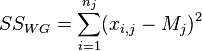
The analysis of variance consists in determining the ratio of systematic (intergroup) variance to random (intragroup) variance in the measured data. The sum of squared deviations of the parameter values from the mean is used as an indicator of variability:  (from the English. Sum of Squares ). It can be shown that the total amount of squares
  decomposed into an intergroup sum of squares
  and intragroup sum of squares
  :
:

Let the exact value of each parameter be its expected value, equal to the average population  . In the absence of systematic errors, the group average and the average of the general population are identical:
  . Then the random measurement error is the difference between the measurement result. and middle groups:
  . If the method
  has a systematic effect, then a systematic error when exposed to this factor is the difference between the average group
  and the average population:
  . Then the equation can be represented as follows:
 , or
, or
 .
.
Then

Where


Consequently

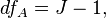
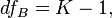
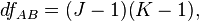
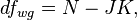
The degrees of freedom are decomposed in the same way:
 Where
Where
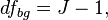
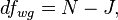
and  is the total sample size, and
  - number of groups.
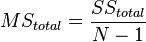
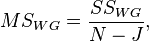
Then the variance of each part, referred to in the analysis of variance model as “average square”, or  (from the English. Mean Square ), is the ratio of the sum of squares to the number of their degrees of freedom:

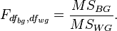
The ratio of intergroup and intragroup dispersions has an F-distribution (Fisher distribution) and is determined using (Fisher's F-test):
The starting points of analysis of variance are
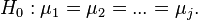
The null hypothesis in the analysis of variance is the statement about the equality of the mean values:
When the null hypothesis is rejected, an alternative hypothesis is accepted that not all averages are equal, that is, there are at least two groups that differ in mean values:

 ≠
≠  ≠
≠  ≠
≠ 
If there are three or more groups, post-hoc t-tests or the method of contrasts are used to determine differences between averages.
The simplest case of analysis of variance is one-dimensional univariate analysis for two or more independent groups, when all groups are combined according to one sign. The analysis verifies the null hypothesis of equality of averages. When analyzing two groups, analysis of variance is identical to the two-sample Student's t-test for independent samples, and the F-statistic is equal to the square of the corresponding t-statistic.
To confirm the equality of variances, Lieven's test is usually used (Levene's test). In the case of rejection of the hypothesis of equality of variances, the main analysis is not applicable. If the variances are equal, then Fisher's F-criterion is used to estimate the ratio of intergroup and intragroup variability:
If the F-statistic exceeds the critical value, then the null hypothesis is rejected and the conclusion is drawn about the inequality of the means. When analyzing the means of the two groups, the results can be interpreted immediately after applying the Fisher criterion.
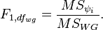
If there are three or more groups, paired comparison of averages is required to identify statistically significant differences between them. A priori analysis includes the method of contrasts, in which the intergroup sum of squares is split into sums of squares of individual contrasts:

Where  there is a contrast between the means of the two groups, and then using the Fisher test, the ratio of the mean square for each contrast to the intragroup mean square is checked:
A posteriori analysis includes post-hoc t-criteria according to Bonferroni or Scheffe methods, as well as a comparison of mean differences by Tukey's method. A special feature of post-hoc tests is the use of an intragroup mean square.  to evaluate any pairs of averages. Tests on the Bonferroni and Scheffe methods are the most conservative since they use the smallest critical area for a given level of significance.
  .
.
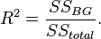
In addition to evaluating the averages, analysis of variance includes determining the coefficient of determination  which shows how much of the total variability is explained by this factor:
Multivariate analysis allows you to check the effect of several factors on a dependent variable. The linear model of the multifactor model is
 ,
,
Where:
 - measurement result th parameter; - average for th parameter; - systematic measurement error -th parameter in
  group by method
  ;
; - systematic measurement error -th parameter in
  group by method
  ;
; - systematic measurement error -th parameter in
  group due to combination of methods and ;
 - random measurement error th parameter.
In contrast to the single-factor model, where there is one intergroup sum of squares, the model of multivariate analysis includes the sum of squares for each factor separately and the sum of squares of all interactions between them. Thus, in a two-factor model, the intergroup sum of squares is decomposed into the sum of squares of the factor , sum of squares of a factor and the sum of squares of interaction factors and :

Accordingly, the three-factor model includes the sum of the squares of the factor , sum of squares of a factor , sum of squares of a factor  and sums of squares of factor interactions and , and , and , as well as the interaction of all three factors
  :
:

The degrees of freedom are decomposed in a similar way:
 Where
Where
and is the total sample size, - the number of levels (groups) of the factor , but  - the number of levels (groups) of the factor .
The analysis tests several null hypotheses:
:  ; :
; :  ; and :
  for all and
Each hypothesis is tested using the Fisher criterion:
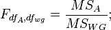
When rejecting the null hypothesis about the influence of a separate factor, the statement is accepted that the main effect of the factor is present. (  etc.). When rejecting the null hypothesis of the interaction of factors, it is assumed that the influence of the factor manifested differently at different levels of the factor . Usually in this case, the results of the general analysis are recognized as invalid, and the influence of the factor checked separately at each factor level using univariate analysis of variance or t-test.
This section contains an introductory overview and discussion of some methods of analysis of variance, including plans with repeated measurements, covariance analysis, multidimensional analysis of variance, unbalanced and nested plans, effects of contrasts, a posteriori comparisons, and others. Additionally, you can refer to evaluation of dispersion components in mixed plans); Experiment planning (sections related to special fields of application of analysis of variance in industrial conditions Viih), as well as Analysis of repeatability and reproducibility (sections relating to the evaluation of the reliability and accuracy of measuring systems).
Main ideas
The purpose of analysis of variance.
The main purpose of analysis of variance is to study the significance of the difference between the averages. The Elementary Concepts of Statistics section contains a brief introduction to the study of statistical significance. If you simply compare the means in two samples, analysis of variance will give the same result as the usual t- criterion for independent samples (if two independent groups of objects or observations are compared) or t- criterion for dependent samples (if two variables are compared on one and the same set of objects or observations). If you are not familiar enough with these criteria, we recommend that you refer to the Basic Statistics section and tables .
Where does the name analysis of variance come from? It may seem strange that the procedure for comparing averages is called variance analysis. In fact, this is due to the fact that when studying the statistical significance of the difference between the averages of two (or several) groups, we actually compare (ie, analyze) the sample variances. The fundamental concept of analysis of variance was proposed by Fisher in 1920. Perhaps the term square-sum analysis or variation analysis would be more natural, but by tradition, the term analysis of variance is used.
See also sections.
See also methods of analysis of variance, components of dispersion and mixed model ANOVA / ANCOVA, as well as the planned experiment.
Splitting the sum of squares
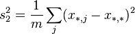
For a sample of volume n, the sample variance is calculated as the sum of the squares of deviations from the sample mean divided by n-1 (sample size minus one).Thus, for a fixed sample size n, the variance is a function of the sum of squares (deviations), denoted, for short, SS (from the English Sum of Squares - Sum of Squares). Then we often omit the word selective, knowing full well that a selective variance or a variance estimate is considered. The basis of analysis of variance is the separation of the dispersion into parts or components. Consider the following data set:
| Group 1 | Group 2 | |
|---|---|---|
| Observation 1 Observation 2 Observation 3 |
2 3 one |
6 7 five |
| The average Sum of Squares (SK) |
2 2 |
6 2 |
| Total average Total sum of squares |
four 28 |
|
The averages of the two groups are significantly different ( 2 and 6, respectively). The sum of the squares of deviations within each group is 2 . Adding them, we get 4. If we now repeat these calculations without taking into account group membership, that is, if we calculate SS based on the total average of these two samples, then we obtain the value 28. In other words, variance (the sum of squares), based on intragroup variability, leads to much smaller values than when calculated on the basis of total variability (relative to the total average). The reason for this, obviously, lies in the significant difference between the average values, and this difference between the average and explains the existing difference between the sums of squares. Indeed, if we use the analysis of variance for the analysis of this data , the following table will be obtained, which is called the analysis of variance table:
| MAIN EFFECT | |||||
|---|---|---|---|---|---|
| SS | st.Sv. | MS | F | p | |
| Effect Mistake |
24.0 4.0 |
one four |
24.0 1.0 |
24.0 | .008 |
As can be seen from the table, the total sum of squares SS = 28 is divided into components: the sum of squares due to intragroup variability ( 2 + 2 = 4 ; see the second row of the table) and the sum of squares due to the difference in mean values between groups (28- (2+ 2) = 24; see the first row of the table). Note that MS in this table is an average square, equal to SS, divided by the number of degrees of freedom (st. Sv).
SS errors and SS effect. Intra-group variability ( SS ) is commonly referred to as residual component or error variance . This means that usually during an experiment it cannot be predicted or explained. On the other hand, the SS effect (or the component of the variance between groups) can be explained by the difference between the average values in the groups. In other words, belonging to a certain group explains intergroup variation, since we know that these groups have different mean values.
Validation. The basic ideas of checking statistical significance are discussed in the Elementary Concepts of Statistics section . The same section explains the reasons why many criteria use the ratio of explained and unexplained variance. An example of such use is analysis of variance itself. The verification of significance in analysis of variance is based on a comparison of the component of the dispersion due to the intergroup spread (called the mean square of the effect or MS effect ) and the component of the dispersion caused by the intragroup spread (called the mean square of the error or MS error; these terms were first used in Edgeworth, 1885). If the null hypothesis is true (the equality of the means in the two populations), then a comparatively small difference in the sample means can be expected due to purely random variability. Therefore, under the null hypothesis, the intra-group variance will almost coincide with the total variance, calculated without regard to group membership. The obtained intragroup dispersions can be compared using the F-test, which checks whether the ratio of dispersions is significantly more than 1. In the above example, the F- test shows that the difference between the means is statistically significant (significant at 0.008).
The basic logic of analysis of variance. Summing up, it can be said that the purpose of analysis of variance is to check the statistical significance of the difference between means (for groups or variables). This check is performed by splitting the sum of squares into components, i.e. by splitting the total variance (variation) into parts, one of which is due to random error (that is, intragroup variability), and the second is related to the difference in mean values. The last component of the variance is then used to analyze the statistical significance of the difference between the mean values. If this difference is significant , the null hypothesis is rejected and an alternative hypothesis is made about the existence of a difference between the means.
Dependent and independent variables. Variables whose values are determined by measurements during an experiment (for example, the score gained during testing) are called dependent variables. Variables that can be controlled during an experiment (for example, teaching methods or other criteria that allow to divide observations into groups or classify) are called factors or independent variables. These concepts are described in more detail in the Elementary Concepts of Statistics section .
Multivariate analysis of variance
В рассмотренном выше простом примере вы могли бы сразу вычислить t- критерий для независимых выборок, используя соответствующую опцию модуля Основные статистики и таблицы. Полученные результаты, естественно, совпадут с результатами дисперсионного анализа. Однако дисперсионный анализ содержит гораздо более гибкие и мощные технические средства, позволяющие исследовать планы практически неограниченной сложности.
Множество факторов. Мир по своей природе сложен и многомерен. Ситуации, когда некоторое явление полностью описывается одной переменной, чрезвычайно редки. Например, если мы пытаемся научиться выращивать большие помидоры, следует рассматривать факторы, связанные с генетической структурой растений, типом почвы, освещенностью, температурой и т.д. Таким образом, при проведении типичного эксперимента приходится иметь дело с большим количеством факторов. Основная причина, по которой использование дисперсионного анализа предпочтительнее повторного сравнения двух выборок при разных уровнях факторов с помощью серий t- критерия, заключается в том, что дисперсионный анализ существенно более эффективен и, для малых выборок, более информативен. Вам нужно сделать определенные усилия, чтобы овладеть техникой дисперсионного анализа, реализованной на STATISTICA, и ощутить все ее преимущества в конкретных исследованиях.
Управление факторами. Предположим, что в рассмотренном выше примере анализа двух выборок мы добавим еще один фактор, например, Пол - Gender . Пусть каждая группа теперь состоит из 3 мужчин и 3 женщин. План этого эксперимента можно представить в виде таблицы 2 на 2:
| Экспериментальная группа 1 |
Экспериментальная группа 2 |
|
|---|---|---|
| Мужчины |
2 3 one |
6 7 five |
| The average | 2 | 6 |
| Женщины |
four five 3 |
eight 9 7 |
| The average | four | eight |
До проведения вычислений можно заметить, что в этом примере общая дисперсия имеет, по крайней мере, три источника: (1) случайная ошибка (внутригрупповая дисперсия), (2) изменчивость, связанная с принадлежностью к экспериментальной группе, и (3) изменчивость, обусловленная полом объектов наблюдения. (Отметим, что существует еще один возможный источник изменчивости - взаимодействие факторов , который мы обсудим позднее). Что произойдет, если мы не будем включать пол как фактор при проведении анализа и вычислим обычный t -критерий? Если мы будем вычислять суммы квадратов, игнорируя пол (т.е. объединяя объекты разного пола в одну группу при вычислении внутригрупповой дисперсии и получив при этом сумму квадратов для каждой группы равную SS =10 и общую сумму квадратов SS = 10+10 = 20), то получим большее значение внутригрупповая дисперсии, чем при более точном анализе с дополнительным разбиением на подгруппы по полу (при этом внутригрупповые средние будут равны 2, а общая внутригрупповая сумма квадратов равна SS = 2+2+2+2 = 8).
So, with the introduction of an additional factor: gender , the residual dispersion decreased. This is due to the fact that the average value for men is less than the average value for women , and this difference in average values increases the total intragroup variability if the gender factor is not taken into account. Controlling error variance increases the sensitivity (power) of the criterion. This example shows another advantage of analysis of variance compared to the usual t- criterion for two samples. Variance analysis allows you to study each factor, controlling the values of other factors. This, in fact, is the main reason for its greater statistical power (for obtaining meaningful results, smaller sample sizes are required). For this reason, analysis of variance, even on small samples, gives statistically more significant results than a simple t- test.
Interaction effects
There is another advantage of variance analysis over the usual t- criterion: analysis of variance allows you to detect the interaction effects between factors and, therefore, allows you to test more complex hypotheses. Consider another example that illustrates what has just been said. (The term interaction was first used by Fisher in Fisher, 1926)
The main effects are pairwise (two-factor) interactions. Suppose that there are two groups of students, and psychologically, students of the first group are set to perform assigned tasks and more purposeful than students of the second group, consisting of more lazy students. We will divide each group randomly in half and offer one half in each group a difficult task, and the other - an easy one. After that, we measure how hard the students work on these tasks. The average values for this (fictional) research are shown in the table:
| Purposeful | Lazy | |
|---|---|---|
| Difficult task Easy task |
ten five |
five ten |
What conclusion can be drawn from these results? Is it possible to conclude that: (1) students work more hard on a difficult task; (2) Ambitious students work harder than lazy ones? None of these statements reflects the essence of the systematic nature of the means given in the table. Analyzing the results, it would be more correct to say that only ambitious students work harder on complex tasks, while only lazy people work harder on light tasks. In other words, the nature of the students and the complexity of the task interacting with each other affect the effort expended. This is an example of pairwise interaction between the character of the students and the complexity of the task. Note that statements 1 and 2 describe the main effects .
Higher order interactions. While pairwise interactions are still relatively easy to explain, higher order interactions are much more difficult to explain. Imagine that in the example above, one more factor was introduced and the following table of averages was obtained:
| Women | Purposeful | Lazy |
|---|---|---|
| Difficult task Easy task |
ten five |
five ten |
| Men | Purposeful | Lazy |
| Difficult task Easy task |
one 6 |
6 one |
What conclusions can now be drawn from the results? Medium plots let you explain complex effects. The analysis of variance module allows you to build these graphs with almost one click. The image on these graphs below represents the three-factor interaction under study.
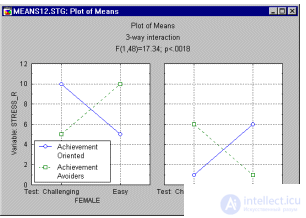
Looking at the graph, we can say that women have an interaction between the nature and complexity of the test: goal-oriented women work on a difficult task more intensely than on a light one. In men, the same interaction is reversed. It can be seen that the description of the interaction between the factors becomes more confusing.
General way of describing interactions. In general, the interaction between factors is described as a change in one effect under the influence of another. In the above example, two-factor interaction can be described as a change in the main effect of a factor characterizing the complexity of a task, under the influence of a factor describing the character of the student. For the interaction of the three factors from the previous paragraph, it can be said that the interaction of the two factors (the complexity of the task and the character of the student) changes under the influence of Paul. If the interaction of four factors is studied, it can be said that the interaction of three factors changes under the influence of the fourth factor, i.e. There are different types of interactions at different levels of the fourth factor. It turned out that in many areas the interaction of five or even more factors is not unusual.
| To the begining |
Difficult plans
In this section, an overview will be given of the main "bricks" from which complex plans are made.
To view other sections of the Introductory Overview, select the appropriate title below.
See also analysis of variance, dispersion components and mixed models ANOVA / ANCOVA and Planning Experiment.
Intergroup and re-measurement plans
When comparing two different groups, the t-criterion for independent samples is usually used (from the Basic Statistics and Tables module). When two variables are compared on the same set of objects (observations), the t- criterion for dependent samples is used. For analysis of variance, sampling is also important or not. If there are repeated measurements of the same variables (under different conditions or at different times) for the same objects , then we speak about the presence of the repeated measurements factor (also called the intragroup factor, since the intragroup sum of squares is calculated to assess its significance). If different groups of objects are compared (for example, men and women, three strains of bacteria, etc.), then the difference between groups is described by an intergroup factor. The methods for calculating the significance criteria for the two types of factors described are different, but their common logic and interpretation coincide.
Inter-and intra-group plans. In many cases, the experiment requires the inclusion in the plan and intergroup factor, and the factor of repeated measurements. For example, the mathematical skills of female and male students (where gender is an intergroup factor) are measured at the beginning and at the end of a semester. Two skills measurements each student form an intragroup factor (or a factor with repeated measurements). Interpretation of the main effects and interactions for intergroup factors and re-measurement factors is the same, and both types of factors can obviously interact with each other (for example, women acquire skills during a semester, and men lose them).
Partial (nested) plans
In many cases, the interaction effect can be neglected. This happens either when it is known that there is no interaction effect in the population, or when the implementation of a full factorial plan is impossible. For example, let the effect of four fuel additives on fuel consumption be studied. Four cars and four drivers are selected. A full factorial experiment requires that each combination — additive, driver, car — appear at least once. To do this, you need at least 4 x 4 x 4 = 64 test groups, which requires too much time. In addition, there is hardly any interaction between the driver and the fuel additive. Taking this into account, you can use a plan like Latin squares, which contains only 16 test groups (four additives are indicated by the letters A, B, C and D):
| Car | ||||
|---|---|---|---|---|
| one | 2 | 3 | four | |
| Driver 1 Driver 2 Driver 3 Driver 4 |
A B C D |
B C D A |
C D A B |
D A B C |
Latin squares are described in most experimental design books (for example, Hays, 1988; Lindman, 1974; Milliken and Johnson, 1984;
продолжение следует...
Часть 1 Variance analysis
Часть 2 - Variance analysis
Нормальность распределения
Предположения. Имеются следующие предположения дисперсионного анализа: зависимая переменная измерена в интервальной шкале (см. раздел Элементарные понятия статистики ); зависимая переменная имеет нормальное распределение внутри каждой группы. Модуль Дисперсионный анализ содержит широкий набор графиков и статистик для проверки этих предположений.
Эффекты нарушения. Вообще F -критерий очень устойчив к отклонению от нормальности (подробнее см. Lindman, 1974). Если эксцесс (см. Основные статистики и таблицы ) больше 0, то значение статистики F может стать очень маленьким. Нулевая гипотеза при этом не может быть отвергнута, хотя она и не верна. Ситуация меняется на противоположную, если эксцесс меньше 0. Асимметрия распределения обычно незначительно влияет на F статистику. Если число наблюдений в ячейке достаточно большое, то отклонение от нормальности не имеет особого значения в силу центральной предельной теоремы , в соответствии с которой, распределение среднего значения при большом объеме выборки близко к нормальному, независимо от начального распределения. Подробное обсуждение устойчивости F статистики можно найти в Box and Anderson (1955) или Lindman (1974).
Однородность дисперсии
Предположения. Предполагается, что дисперсии в разных группах одинаковы. Это предположение называется предположением об однородности дисперсии. Напомним, что в предыдущих разделах описывая вычисление суммы квадратов ошибок мы производили суммирование внутри каждой группы. Если дисперсии в двух группах отличаются друг от друга, то сложение их не естественно и не дает верной оценки общей внутригрупповой дисперсии (так как в этом случае общей дисперсии вообще не существует). Модуль Дисперсионный анализ -ANOVA/MANOVA содержит большой набор статистических критериев, позволяющих обнаружить неоднородность дисперсии.
Эффекты нарушения. Линдман (Lindman 1974, стр. 33) показывает, что F критерий вполне устойчив относительно нарушения предположений однородности дисперсии (см. также Box, 1954a, 1954b; Hsu, 1938).
Специальный случай: коррелированность средних и дисперсий. Бывают случаи, когда F статистика может вводить в заблуждение. Это бывает, когда в ячейках плана средние значения коррелированы с дисперсией. Модуль Дисперсионный анализ позволяет строить диаграммы рассеяния дисперсии или стандартного отклонения относительно средних для обнаружения такой корреляции. Причина, по которой такая корреляция опасна, состоит в следующем. Представим себе, что имеется 8 ячеек в плане, 7 из которых имеют почти одинаковое среднее, а в одной ячейке среднее намного больше остальных. Тогда F критерий может обнаружить статистически значимый эффект. Но предположим, что в ячейке с большим средним значением и дисперсия значительно больше остальных, т.е. среднее значение и дисперсия в ячейках зависимы (чем больше среднее, тем больше дисперсия). В этом случае большое среднее значение ненадежно, так как оно может быть вызвано большой дисперсией данных. Однако F статистика, основанная на объединенной дисперсии внутри ячеек, будет фиксировать большое среднее, хотя критерии, основанные на дисперсии в каждой ячейке не все различия в средних будут считать значимыми.
Такой характер данных (большое среднее и большая дисперсия) часто встречается, когда имеются резко выделяющиеся наблюдения. Одно или два резко выделяющихся наблюдений сильно смещают среднее значение и очень увеличивают дисперсию.
Однородность дисперсии и ковариаций
Предположения. В многомерных планах, с многомерными зависимыми измерениями, также применяются предположение об однородности дисперсии, описанные ранее. Однако так как существуют многомерные зависимые переменные, то требуется так же чтобы их взаимные корреляции (ковариации) были однородны по всем ячейкам плана. Модуль Дисперсионный анализ предлагает разные способы проверки этих предположений.
Эффекты нарушения. Многомерным аналогом F- критерия является лямбда-критерий Уилкса. Не так много известно об устойчивости (робастности) лямбда-критерия Уилкса относительно нарушения указанных выше предположений. Тем не менее, так как интерпретация результатов модуля Дисперсионный анализ основывается обычно на значимости одномерных эффектов (после установления значимости общего критерия), обсуждение робастности касается, в основном, одномерного дисперсионного анализа. Поэтому должна быть внимательно исследована значимость одномерных эффектов.
Специальный случай:ковариационный анализ. Особенно серьезные нарушения однородности дисперсии/ковариаций могут происходить, когда в план включаются ковариаты. В частности, если корреляция между ковариатами и зависимыми измерениями различна в разных ячейках плана, может последовать неверное истолкование результатов. Следует помнить, что в ковариационном анализе, в сущности, проводится регрессионный анализ внутри каждой ячейки для того, чтобы выделить ту часть дисперсии, которая соответствует ковариате. Предположение об однородности дисперсии/ковариации предполагает, что этот регрессионный анализ проводится при следующем ограничении: все регрессионные уравнения (наклоны) для всех ячеек одинаковы. Если это не выполняется, могут появиться большие ошибки. Модуль Дисперсионный анализ имеет несколько специальных критериев для проверки этого предположения. Можно посоветовать использовать эти критерии, для того, чтобы убедиться, что регрессионные уравнения для различных ячеек примерно одинаковы.
Сферичность и сложная симметрия
Причины использования многомерного подхода к повторным измерениям в дисперсионном анализе. В планах, содержащих факторы повторных измерений с более чем двумя уровнями, применение одномерного дисперсионного анализа требует дополнительных предположений: предположения о сложной симметрии и о сферичности . Эти предположения редко выполняются (см. ниже). Поэтому в последние годы многомерный дисперсионный анализ завоевал популярность в таких планах (оба подхода совмещены в модуле Дисперсионный анализ ). Предположение о сложной симметрии состоит в том, что дисперсии (общие внутригрупповые) и ковариации (внутри групп) для различных повторных измерений однородны (одинаковы). Это достаточное условие для того, чтобы одномерный F критерий для повторных измерений был обоснованным (т.е. выданные F-значения в среднем соответствовали F -распределению). Однако, в данном случае, это не условие не является необходимым. Условие сферичности является необходимым и достаточным условием для обоснованного применения F-критерия. Смысл условия состоит в том, что внутри групп все наблюдения должны быть независимы и одинаково распределены. Природа этих предположений, а также влияние их нарушений обычно не очень хорошо описаны в книгах по дисперсионному анализу. Мы даем это описание в следующих параграфах. Там же будет показано, что результаты одномерного подхода могут отличаться от результатов многомерного подхода, и будет объяснено, что это означает.
Необходимость независимости гипотез. Общий способ анализа данных в дисперсионном анализе - это подгонка модели . Если относительно модели, соответствующей данным, имеются некоторые априорные гипотезы, то дисперсия разбивается для проверки этих гипотез (проверка главных эффектов, взаимодействий). С вычислительной точки зрения этот подход строит некоторое множество контрастов (множество сравнений средних в плане). Однако если контрасты не независимы друг от друга, то разбиение дисперсии на компоненты не имеет смысла. Например, если два контраста A и B тождественны, то соответственная им компонента дисперсии выделяется дважды. Например, глупо и бессмысленно выделять две гипотезы: "среднее в ячейке 1 выше среднего в ячейке 2" и "среднее в ячейке 1 выше среднего в ячейке 2". Итак, гипотезы должны быть независимы или ортогональны (термин ортогональность впервые использован в работе Yates, 1933).
Независимые гипотезы при повторных измерениях. Общий алгоритм, реализованный в модуле Дисперсионный анализ , будет пытаться для каждого эффекта генерировать независимые (ортогональные) контрасты (см. раздел Технические замечания руководства пользователя). Для фактора повторных измерений эти контрасты задают множество гипотез относительно разностей между уровнями рассматриваемого фактора. Однако если эти разности коррелированы внутри групп, то результирующие контрасты не являются больше независимыми. Например, в обучении, где обучающиеся измеряются три раза за один семестр, может случиться, что изменения между 1 и 2 измерением отрицательно коррелируют с изменением между 2 и 3 измерениями субъектов. Те, кто большую часть материала освоил между 1 и 2 измерениями, осваивают меньшую часть в течение того времени, которое прошло между 2 и 3 измерением. В действительности, для большинства случаев, где дисперсионный анализ используются при повторных измерениях, можно предположить, что изменения по уровням коррелированы по субъектам. Однако когда это происходит, предположение о сложной симметрии и сферичности не выполняются и независимые контрасты не могут быть вычислены.
Влияние нарушений и способы их исправления. Когда предположения о сложной симметрии или о сферичности не выполняются, дисперсионный анализ может выдать ошибочные результаты. До того, как были достаточно разработаны многомерные процедуры, было предложено несколько предположений для компенсации нарушений этих предположений. (См., например, работы Greenhouse & Geisser, 1959 и Huynh & Feldt, 1970). Эти методы до сих пор широко используются (поэтому они представлены в модуле Дисперсионный анализ ).
Подход многомерного дисперсионного анализа к повторным измерениям. В целом проблемы сложной симметрии и сферичности относятся к тому факту, что множества контрастов, включенных в исследование эффектов факторов повторных измерений (с числом уровней больше двух) не независимы друг от друга. Однако им не обязательно быть независимыми, если используется многомерный критерий для одновременной проверки статистического значимости двух или более контрастов фактора повторных измерений. Это является причиной того, что методы многомерного дисперсионного анализа стали чаще использоваться для проверки значимости факторов одномерных повторных измерений с более чем 2 уровнями. Этот подход широко распространен, так как он, в общем случае, не требует предположения о сложной симметрии и предположения о сферичности.
Случаи, в которых подход многомерного дисперсионного анализа не может быть использован. Существуют примеры (планы), когда подход многомерного дисперсионного анализа не может быть применен. Обычно это случаи, когда имеется небольшое количество субъектов в плане и много уровней в факторе повторных измерений. Тогда для проведения многомерного анализа может быть слишком мало наблюдений. Например, если имеется 12 субъектов, p = 4 фактора повторных измерений, и каждый фактор имеет k = 3 уровней. Тогда взаимодействие 4-х факторов будет "расходовать" (k-1)p = 24 = 16 степеней свободы. Однако имеется лишь 12 субъектов, следовательно, в этом примере многомерный тест не может быть проведен. Модуль Дисперсионный анализ самостоятельно обнаружит эти наблюдения и вычислит только одномерные критерии.
Различия в одномерных и многомерных результатах. Если исследование включает большое количество повторных измерений, могут возникнуть случаи, когда одномерный подход дисперсионного анализа к повторным измерениям дает результаты, сильно отличающиеся от тех, которые были получены при многомерном подходе. Это означает, что разности между уровнями соответствующих повторных измерений коррелированы по субъектам. Иногда этот факт представляет некоторый самостоятельный интерес.
Методы дисперсионного анализа
Методы дисперсионного анализа обсуждаются в нескольких разделах этого учебника. Хотя многие из доступных статистических методов описываются одновременно в нескольких главах, каждый из них наиболее удобен при работе в определенной области приложений.
Диспресионный анализ: Эта глава включает обзор полнофакторных планов, планов с повторными измерениями, планов многомерного дисперсионного и ковариационного анализа (MANOVA), планов с балансированной вложенностью (планы бывают не сбалансированными, т.е. имеющими различные размеры выборок n при некоторых испытаниях), а также описание оцениванияспланированных и апостериорных сравнений и мн. others
Компоненты дисперсии и смешанная модель ANCOVA: Эта глава включает обсуждение экспериментов со случайными эффектами (смешанная модель дисперсионного анализ), оцениваниекомпонент дисперсии для случайных эффектов, планов с большими главными эффектами (например, с факторами, имеющими более 100 уровней) с/без случайных эффектов, а также в случае планов с большим числом факторов, когда необходимо оценить все взаимодействия.
Планирование эксперимента: Эта глава включает обсуждение стандартных экспериментальных планов, используемых в промышленных/производственных приложениях, включая 2**(kp) и3**(kp) планы, центральные композиционные и нефакторные планы, планы для смесей, D- и A-оптимальные планы, а также планы для произвольных ограниченных областей значений экспериментальных данных.
Анализ повторяемости и воспроизводимости (в главе Анализ процессов ): Этот раздел главы Анализ процессов включает обсуждение планов специального вида, используемых для оценивания надежности и точности измерительных устройств; Эти планы обычно включают два или три случайных фактора и набор специализированных статистик, позволяющих оценить качество измерительной системы (обычно в промышленных/производственных приложениях).
Таблицы группировки (в главе Основные статистики и таблицы): Эта глава включает обсуждение экспериментов, одного (многоуровневого) или нескольких (любых) факторов в случаях, когда не требуется проведение полного дисперсионного анализа.
| To the begining |

Comments
To leave a comment
Probability theory. Mathematical Statistics and Stochastic Analysis
Terms: Probability theory. Mathematical Statistics and Stochastic Analysis