Lecture
The normal distribution law (often called the Gauss law) plays an extremely important role in probability theory and occupies a special position among other distribution laws. This is the most common distribution law in practice. The main feature that distinguishes a normal law from other laws is that it is a limiting law, to which other laws of distribution approach under typical conditions that are very often encountered.
It can be proved that the sum of a sufficiently large number of independent (or weakly dependent) random variables, subject to arbitrary distribution laws (subject to certain very non-rigid restrictions), approximately obeys the normal law, and this is done more accurately the more random variables are summed. Most of the random variables encountered in practice, such as measurement errors, shooting errors, etc., can be represented as sums of a very large number of relatively small terms — elementary errors, each of which is caused by a separate cause independent of the others. . Whatever distribution laws are subject to individual elementary errors, the features of these distributions in the sum of a large number of terms are leveled, and the sum turns out to be subject to a law that is close to normal. The main restriction imposed on the summable errors is that they all play a relatively small role in the total amount. If this condition is not fulfilled and, for example, one of the random errors turns out to be in its effect on the sum sharply prevailing over all others, then the distribution law of this prevailing error will impose its influence on the sum and determine its distribution law in basic features.
Theorems that establish a normal law as a limit for the sum of independent uniformly small random terms will be discussed in more detail in Chapter 13.
The normal distribution law is characterized by the probability density of the form:
 (6.1.1)
The distribution curve according to the normal law has a symmetric hilly-like appearance (Fig. 6.1.1). The maximum ordinate of the curve is equal to  corresponding to point
  ; as the distance from the point
  distribution density falls, and at
  the curve asymptotically approaches the abscissa axis.
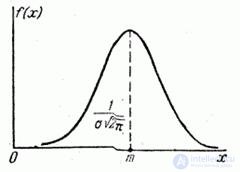
Fig. 6.1.1.
Find out the meaning of numerical parameters and  included in the expression of the normal law (6.1.1); prove that magnitude is nothing but the expectation, and the magnitude - standard deviation of magnitude
  . To do this, we calculate the basic numerical characteristics of - expectation and variance.

Using variable substitution

we have:
 (6.1.2)
It is easy to verify that the first of the two intervals in formula (6.1.2) is zero; the second is the famous Euler-Poisson integral:
 . (6.1.3)
Consequently,
 ,
,
those. parameter is the expected value of . This parameter, especially in firing tasks, is often referred to as the center of dispersion (abbreviated as c. P.).
Calculate the variance of the value :
 .
.
Using the change variable again
we have:
 .
.
Integrating in parts, we get:
 .
.
The first term in braces is zero (since  at
at  decreases faster than any degree increases
  ), the second term by the formula (6.1.3) is equal to
  from where
 .
.
Therefore, the parameter in the formula (6.1.1) there is nothing more than the standard deviation of .
Find out the meaning of the parameters and normal distribution. Directly from formula (6.1.1) it can be seen that the center of symmetry of the distribution is the center of dispersion . This is clear from the fact that when the difference sign changes  the inverse expression (6.1.1) does not change. If you change the center of dispersion , the distribution curve will shift along the abscissa axis, without changing its shape (Fig. 6.1.2). The center of dispersion characterizes the position of the distribution on the x-axis.
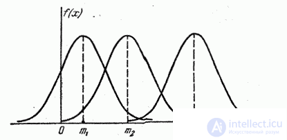
Fig. 6.1.2.
The dimension of the center of dispersion is the same as the dimension of a random variable. .
Parameter characterizes not the position, but the very form of the distribution curve. This is the dispersion characteristic. The largest ordinate of the distribution curve is inversely proportional ; while increasing maximum ordinate decreases. Since the area of the distribution curve should always remain equal to unity, then with increasing the distribution curve becomes flatter, stretching along the abscissa; on the contrary, while decreasing the distribution curve stretches upward, simultaneously contracting from the sides, and becomes more needle-like. In fig. 6.1.3 three normal curves are shown (I, II, III) with  ; of these, curve I corresponds to the largest, and curve III to the smallest . Parameter change equivalent to a change in the scale of the distribution curve — an increase in the scale along one axis and a similar decrease along the other.
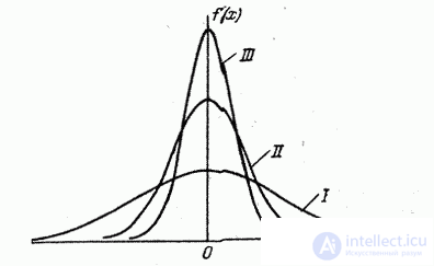
Fig. 6.1.3.
Dimension parameter naturally coincides with the dimension of a random variable .
In some probability theory courses, the so-called measure of accuracy is used instead of the standard deviation as the characteristic of dispersion for a normal law. A measure of accuracy is a quantity inversely proportional to the standard deviation. :
 .
.
The dimension of the measure of accuracy is the inverse of the dimension of a random variable.
The term “measure of accuracy” is borrowed from the theory of measurement errors: the more accurate the measurement, the greater the measure of accuracy. Using the measure of accuracy  You can write a normal law in the form:
 .
.

Comments
To leave a comment
Probability theory. Mathematical Statistics and Stochastic Analysis
Terms: Probability theory. Mathematical Statistics and Stochastic Analysis