5.2. Distribution function

In the previous section, we introduced the distribution series as an exhaustive characteristic (distribution law) of a discontinuous random variable. However, this characteristic is not universal; it exists only for discontinuous random variables. It is easy to verify that such a characteristic cannot be constructed for a continuous random variable. Indeed, a continuous random variable has an infinite number of possible values ​​that completely fill a certain interval (the so-called “countable set”). It is impossible to create a table in which all possible values ​​of such a random variable would be listed. In addition, as we will see later, each individual value of a continuous random variable usually does not have any non-zero probability. Consequently, for a continuous random variable, there is no series of distribution in the sense in which it exists for a continuous quantity. However, different regions of possible values ​​of a random variable are still not equally probable, and for a continuous quantity there is a “probability distribution”, although not in the same sense as for a discontinuous one.

To quantify this probability distribution, it is convenient to use the non-probability of the event. and the probability of an event where - some current variable. The probability of this event obviously depends on , there is some function from . This function is called the distribution function of the random variable. and is denoted by :

. (5.2.1)

Distribution function sometimes also called integral distribution function or integral distribution law.

The distribution function is the most universal characteristic of a random variable. It exists for all random variables: both discontinuous and continuous. The distribution function fully characterizes a random variable from a probabilistic point of view, i.e. is a form of distribution law.

We formulate some general properties of the distribution function.

1. Distribution function there is a non-decreasing function of its argument, i.e. at .

2. At minus infinity, the distribution function is zero: .

3. At plus infinity, the distribution function is equal to one: .

Without giving a rigorous proof of these properties, we illustrate them with a visual geometric interpretation. For this we will consider a random variable. as a random point on the Ox axis (fig. 5.2.1), which as a result of experience may take one or another position. Then the distribution function there is a chance that a random point as a result of the experience will fall to the left of the point .

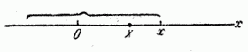
Fig. 5.2.1.

We will increase i.e. move point right on the x-axis. Obviously, with this, the probability that a random point will fall to the left , can not decrease; therefore, the distribution function with increasing can not decrease.

To make sure that , we will move the point indefinitely left on the x-axis. At the same time hit a random point to the left in the limit becomes an impossible event; it is natural to assume that the probability of this event tends to zero, i.e. .

Similarly, moving the point indefinitely right make sure that since the event becomes in the limit authentic.

Distribution function graph in the general case, it is a graph of a non-decreasing function (Fig. 5.2.2), the values ​​of which start from 0 and reach 1, and at certain points the function may have jumps (discontinuities).

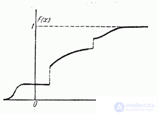
Fig. 5.2.2.

Knowing the distribution number of a discontinuous random variable, one can easily construct the distribution function of this quantity. Really,

,

where inequality under the sum sign indicates that the summation applies to all those values which are smaller .

When is the current variable passes through any of the possible values ​​of the discontinuous value , the distribution function changes abruptly, and the magnitude of the jump is equal to the probability of this value.

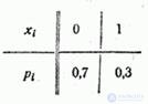
Example 1. One experience is performed in which an event may or may not appear. . Event probability equal to 0.3. Random value - the number of occurrences in experience (characteristic random variable of event ). Build its distribution function.

Decision. Distribution range has the form:

Construct the distribution function of :

1) at

;

2) at

;

3) at

.

The graph of the distribution function is shown in Fig. 5.2.3. At break points function accepts values ​​marked by dots in the drawing (the function is continuous on the left).

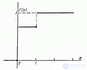
Fig. 5.2.3.

Example 2. In the conditions of the previous example, 4 independent experiments are performed. Build the distribution function of the number of occurrences of the event .

Decision. Denote - the number of occurrences in four experiments. This value has a number of distribution

Construct the distribution function of a random variable :

1) at ;

2) at ;

3) at ;

4) at ;

5) at ;

6) at .

The graph of the distribution function is shown in Fig. 5.2.4.

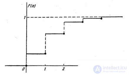
Fig. 5.2.4.

The distribution function of any discontinuous random variable is always a discontinuous step function whose jumps occur at points corresponding to possible random values ​​of the magnitude and are equal to the probabilities of these values. The sum of all function jumps equals one.

As the number of possible values ​​of a random variable increases and the intervals between them jumps, the jumps become larger, and the jumps themselves become smaller; the stepped curve becomes smoother (Fig. 5.2.5); the random value gradually approaches the continuous value, and its distribution function to the continuous function (Fig. 5.2.6).

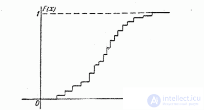
Fig. 5.2.5.

Fig. 5.2.6.

In practice, the distribution function of a continuous random variable is usually a function that is continuous at all points, as shown in Fig. 5.2.6. However, it is possible to construct examples of random variables, the possible values ​​of which continuously fill a certain gap, but for which the distribution function is not everywhere continuous, but at certain points it suffers a discontinuity (Fig. 5.2.7).

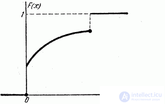
Fig. 5.2.7.

Such random variables are called mixed. As an example of a mixed quantity, we can take the area of ​​damage caused to a target by a bomb whose radius of destructive action is equal to R (Fig. 5.2.8).

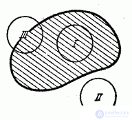
Fig. 5.2.8.

The values ​​of this random variable continuously fill the gap from 0 to , carried out at the positions of a bomb type I and II, have a certain finite probability, and the values ​​of the distribution function correspond to these values, whereas in intermediate values ​​(position of type III) the distribution function is continuous. Another example of a mixed random variable is the time T of the failure-free operation of the device, tested during the time t. The distribution function of this random variable is continuous everywhere except at the point t.