3.2. Probability addition theorem

The probability addition theorem is formulated as follows.

The probability of the sum of two incompatible events is equal to the sum of the probabilities of these events:

. (3.2.1)

Let us prove the probability addition theorem for the case scheme. Let the possible outcomes of the experience be reduced to a set of cases, which, for clarity, we depict in the form of n points:

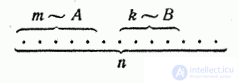
Suppose that of these cases favorable event , but - event . Then

Since the events and incompatible, there are no such cases that are favorable and and together. Therefore, the event favorable cases and

Substituting the obtained expressions into formula (3.2.1), we obtain the identity. The theorem is proved.

Let us generalize the addition theorem to the case of three events. Denoting an event letter , and adding to the amount of another event it is easy to prove that

Obviously, using the full induction method, one can generalize the addition theorem to an arbitrary number of incompatible events. Indeed, suppose that it is valid for n events:

and prove that it will be valid for events:

Denote:

We have:

.

But since for n events we consider the theorem already proved, then

,

from where

,

Q.E.D.

Thus, the addition theorem is applicable to any number of incompatible events. It is more convenient to write in the form:

. (3.2.2)

We point out the consequences arising from the probability addition theorem.

Corollary 1. If events form a complete group of incompatible events, the sum of their probabilities is equal to one:

.

Evidence. Since the events form a complete group, the appearance of at least one of them is a reliable event:

.

Because - incompatible events, the probability addition theorem is applicable to them

,

from where

,

Q.E.D.

Before deriving the second consequence of the addition theorem, we define the concept of "opposing events."

Opposite events are two incompatible events that make up the full group.

Event opposite to event it is customary to denote .

Examples of opposite events.

one) - hit with a shot, - miss when fired;

2) - loss of the coat of arms when throwing a coin, - loss of numbers when throwing a coin;

3) - trouble-free operation of all elements of the technical system, - failure of at least one element;

four) - detection of at least two defective items in the inspection lot, - detection of no more than one defective product.

Corollary 2. The sum of the probabilities of opposite events is equal to one:

.

This consequence is a special case of Corollary 1. It is highlighted especially because of its great importance in the practical application of probability theory. In practice, it is often easier to calculate the probability of the opposite event. than the probability of a direct event . In these cases, calculate and find .

Consider a few examples on the application of the addition theorem and its consequences.

Example 1. There are 1000 tickets in the lottery; 500 rubles are won for one ticket, 100 rubles for 100 tickets, 20 rubles for 50 tickets, 5 rubles for 100 tickets, other tickets are non-winning. Someone buys one ticket. Find the probability of winning at least 20 rubles.

Decision. Consider the events:

- win at least 20 rubles.,

- win 20 rubles.

- win 100 rubles.

- win 500 rubles.

Obviously

.

By the addition theorem

.

Example 2. Three ammunition depots are bombed, one bomb being dropped. The probability of getting into the first warehouse is 0.01; in the second 0,008; in the third 0.025. When hit in one of the warehouses all three explode. Find the probability that the warehouses will be blown up.

Decision. Consider the events:

- explosion of warehouses,

- getting into the first warehouse,

- getting into the second warehouse,

- getting into the third warehouse.

Obviously

.

Since when dropping a single bomb event incompatible then

.

Example 3. The circular target (Fig. 3.2.1) consists of three zones: I, II and III. The probability of hitting the first zone with one shot is 0.15, the second is 0.23, and the third is 0.17. Find the probability of a miss.

Fig. 3.2.1.

Decision. Denote - miss - hit. Then

,

Where - hit respectively in the first, second and third zones

,

from where

.

As already mentioned, the probability addition theorem (3.2.1) is valid only for incompatible events. In the event that events and are joint, the probability of the sum of these events is expressed by the formula

. (3.2.3)

The validity of formula (3.2.3) can be clearly seen by considering Figure 3.2.2.

Fig. 3.2.2.

Similarly, the probability of the sum of three joint events is calculated by the formula

.

The validity of this formula also clearly follows from the geometric interpretation (Fig. 3.2.3).

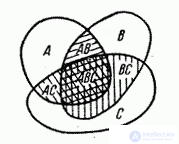
Fig. 3.2.3.

The method of complete induction can prove the general formula for the probability of the sum of any number of joint events:

, (3.2.4)

where amounts apply to different index values , etc.

Formula (3.2.4) expresses the probability of the sum of any number of events in terms of the probabilities of the products of these events, taken one, two, three, etc.

A similar formula can be written for the production of events. Indeed, from fig. 3.2.2 it is immediately clear that

. (3.2.5)

From fig. 3.2.3 shows that

. (3.2.6)

The general formula expressing the probability of the product of an arbitrary number of events in terms of the probabilities of the sums of these events, taken one, two, three, etc., has the form:

. (3.2.7)

Formulas of the type (3.2.4) and (3.2.7) find practical application in converting various expressions containing probabilities of sums and products of events. Depending on the specifics of the task, in some cases it is more convenient to use only sums, and in others only the works of events: similar formulas serve to convert one into another.

Example. The technical device consists of three units: two units of the first type - and - and one unit of the second type - . Aggregates and duplicate each other: if one of them fails, it automatically switches to the second. Unit not duplicated. In order for the device to stop working (failed), it is necessary that both units fail simultaneously. and or unit . Thus, a device failure is an event. - is presented in the form:

,

Where - unit failure , - unit failure , - unit failure .

Required to express the probability of an event through probabilities of events that contain only sums, and not products of elementary events , and .

Decision. By the formula (3.2.3) we have:

; (3.2.8)

according to the formula (3.2.5)

;

according to the formula (3.2.6)

.

Substituting these expressions into (3.2.8) and making abbreviations, we get:

.