Lecture
With a large number of observations (of the order of hundreds), a simple statistical aggregate ceases to be a convenient form of recording statistical material — it becomes too cumbersome and little visual. To make it more compact and clear, the statistical material should be subjected to additional processing - the so-called “statistical series” is built.
Suppose that at our disposal the results of observations on a continuous random variable  , decorated in the form of a simple statistical aggregate. Divide the entire range of observed values. at intervals or "digits" and count the number of values
  attributable to each
  th digit This number is divided by the total number of observations.
  and find the frequency corresponding to this category:
 . (7.3.1)
The sum of the frequencies of all bits, obviously, should be equal to one.
We construct a table in which the discharges are given in the order of their location along the abscissa axis and the corresponding frequencies. This table is called a statistical series:
|
|
|
|
|
|
|
|
|
|
|
|
|
|
Here  - designation
  th discharge
  - its boundaries;
  - appropriate frequency;
  - number of digits.
Example 1. 500 measurements of lateral aiming errors were made when shooting from a plane at a ground target. The measurement results (in thousandths of radians) are summarized in a statistical series:
| -four; -3 | -3; -2 | -2; -one | -one; 0 | 0; one | one; 2 | 2; 3 | 3; four |
| 6 | 25 | 72 | 133 | 120 | 88 | 46 | ten |
| 0.012 | 0.050 | 0.144 | 0.266 | 0.240 | 0.176 | 0.092 | 0.020 |
Here indicated intervals of error values; - the number of observations in this interval,  - appropriate frequencies.
When the observed values of a random variable are grouped by digits, the question arises as to which digit to assign a value that is exactly on the border of two digits. In these cases, we can recommend (purely arbitrary) to consider this value as belonging to both digits and add to the numbers of one and another category  .
.
The number of digits into which statistical material should be grouped should not be too large (then the distribution series becomes inexpressive and irregular oscillations are detected in it); on the other hand, it should not be too small (with a small number of digits, the distribution properties are described by the statistical series too roughly). Practice shows that in most cases it is rational to choose the number of digits of the order of 10 to 20. The richer and more homogeneous the statistical material, the greater the number of digits that can be chosen when drawing up the statistical series. The lengths of the discharges may be the same or different. Easier, of course, to take them the same. However, when drawing up data on random variables that are distributed extremely non-uniformly, it is sometimes convenient to choose narrower discharges in the region of the highest distribution density than in the region of low density.
The statistical series is often drawn up graphically in the form of a so-called histogram. The histogram is constructed as follows. Discharges are deposited along the abscissa, and a rectangle is constructed on each of the discharges as their base, the area of which is equal to the frequency of the discharge. To construct a histogram, the frequency of each digit should be divided by its length and the resulting number taken as the height of the rectangle. In the case of equal length discharges, the heights of the rectangles are proportional to the corresponding frequencies. From the method of constructing a histogram, it follows that its total area is equal to one.
As an example, one can cite a histogram for the pickup error, constructed according to the statistical series considered in Example 1 (Fig. 7.3.1).
Obviously, with an increase in the number of experiments, it is possible to choose smaller and smaller discharges; at the same time, the histogram will increasingly approach a certain curve that bounds an area equal to one. It is easy to verify that this curve is a plot of the density distribution .
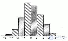
Fig. 7.3.1
Using the data of the statistical series, it is possible to construct approximately the statistical distribution function of . Construction of an exact statistical distribution function with several hundred jumps in all observed values too laborious and does not justify itself. For practice, it is usually sufficient to construct a statistical distribution function at several points. As these points it is convenient to take the boundaries  discharges that appear in the statistical series. Then obviously
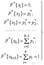 (7.3.2)
Combining the obtained points with a broken line or a smooth curve, we obtain an approximate graph of the statistical distribution function.
Example 2. Construct an approximate statistical distribution function of the error of a tip according to the statistical series of Example 1.

Fig. 7.3.2
Decision. Using formulas (7.3.2), we have:

An approximate graph of the statistical distribution function is given in Fig. 7.3.2.


Comments
To leave a comment
Probability theory. Mathematical Statistics and Stochastic Analysis
Terms: Probability theory. Mathematical Statistics and Stochastic Analysis