14.5. Frequency probability estimate

In practice, it is often necessary to estimate an unknown probability. developments by its frequency at independent experiences.

This task is closely related to those considered in the previous ones. . Indeed, the frequency of the event at independent experiments is nothing more than the arithmetic average of the observed values ​​of which in each individual experience takes the value 1 if the event appeared, and 0, if not appeared:

. (14.5.1)

Recall that the expected value equally ; its dispersion where . The mathematical expectation of the arithmetic mean is also equal to

(14.5.2)

i.e. assessment for is unbiased.

Variance of magnitude equals

. (14.5.3)

It is possible to prove that this variance is minimally possible, i.e. for is effective.

Thus, as a point estimate for an unknown probability it is reasonable to take frequency in all cases . The question arises about the accuracy and reliability of such an assessment, i.e., about building a confidence interval for the probability .

Although this problem is a special case of the previously considered confidence interval problem for mathematical expectation, it is still advisable to solve it separately. The specificity here is that the magnitude - a discontinuous random variable with only two possible values: 0 and 1. In addition, its expectation and variance linked by functional dependence. This simplifies the task of building a confidence interval.

We first consider the simplest case, when the number of experiments relatively high and the probability not too big and not too small. Then we can assume that the frequency of the event there is a random variable whose distribution is close to normal. Calculations show that this assumption can be used even for not very large values. : enough for both quantities and there were more than four. We will assume that these conditions are met and the frequency can be considered distributed according to the normal law. The parameters of this law will be:

; . (14.5.4)

Suppose first that the quantity we know. Assign confidence probability and find such an interval to value fell into this interval with probability :

. (14.5.5)

Since the value distributed normally then

,

from where as in 14.3,

,

Where - inverse function of the normal distribution function .

For determining , As in 14.3, can be denoted

.

Then

, (14.5.6)

Where determined from table 14.3.1.

So with probability it can be argued that

. (14.5.7)

Actual value unknown to us; however, inequality (14.5.7) will have the probability regardless of whether we know or do not know the probability . Getting from experience a specific frequency value , it is possible, using inequality (14.5.7), to find the interval which with probability covers the point . Indeed, we transform this inequality to the form

(14.5.8)

and give it a geometric interpretation. We will postpone the frequency on the x-axis and the ordinate is the probability (fig. 14.5.1).

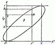
Fig. 14.5.1.

Geometric location of points whose coordinates and satisfy the inequality (14.5.8), will be the inner part of the ellipse passing through the points and and having tangents at these points parallel to the axis . Since the value there can be neither negative nor greater than one, then the region corresponding to inequality (14.5.8), it is necessary to restrict left and right straight lines and . Now possible for any value obtained from experience, build a confidence interval which with probability will cover an unknown value . For this we draw through the point straight line parallel to the ordinate axis; on this straight border area will cut off the confidence interval . Really point with random abscissa and non-random (but unknown) ordinate with probability gets inside the ellipse, i.e. spacing with probability will cover the point .

The size and configuration of the “confidence ellipse” depends on the number of experiments. . The more , the more the ellipse is stretched and the narrower the confidence interval.

Confidence limits and can be found from relation (14.5.8), replacing the inequality sign with equality. Solving the resulting quadratic equation with respect to , we get two roots:

(14.5.9)

Confidence interval for probability will be

.

Example 1. Event frequency in a series of 100 experiments was . Determine the 90% confidence interval for the probability. developments .

Decision. First of all, we check the applicability of the normal law; for this we estimate the values and . Assuming roughly get

; .

Both values ​​are much greater than four; normal law is applicable. From table 14.3.1 for we find . By the formulas (14.5.9) we have

; ; .

Note that when increasing magnitudes and in formulas (14.5.9) tend to zero; in the limit, the formulas take the form

(14.5.10)

These formulas can also be obtained directly by using the approximate method of constructing a confidence interval for the expectation given in 14.3. Formulas (14.5.10) can be used for large (on the order of hundreds), if only the probability not too large and not too small (for example, when both quantities are and about 10 or more).

Example 2. Made 200 experiments; event frequency turned out to be . Construct an 85% confidence interval for the probability of an event approximately (using formulas (14.5.10)). Compare the result with the exact corresponding formulas (14.5.9).

Decision. ; according to table 14.3.1 we find . Multiplying it by

,

will get

,

where do we find the approximate confidence interval

.

By the formulas (14.5.9) we find more accurate values. ; which almost do not differ from the approximate.

Above, we considered the question of constructing a confidence interval for the case of a sufficiently large number of experiments where the frequency can be considered normally distributed. With a small number of experiments (and also if the probability very large or very small) such an assumption cannot be used. In this case, the confidence interval is built based not on the approximate, but on the exact law of frequency distribution. It is easy to verify that this is the binomial distribution discussed in Chapters 3 and 4. Indeed, the number of occurrences of an event at experiments are distributed according to the binomial law: the probability that an event will appear exactly times equals

, (14.5.11)

and frequency there is nothing more than the number of occurrences of an event divided by the number of experiences.

Based on this distribution, you can build a confidence interval similar to the way we built it, based on the normal law for large (p. 331).

Suppose first that the probability we know and find the frequency range , in which with probability event frequency .

For the case of large we used the normal distribution law and took an interval symmetric with respect to the expectation. The binomial distribution (14.5.11) does not have symmetry. In addition, (due to the fact that the frequency is a discontinuous random variable) of the interval, the probability of hitting it is exactly equal to may not exist. Therefore, we choose as the interval , the smallest interval, the probability of falling to the left of which and to the right of which will be greater .

Similar to the way we built the area for a normal law (fig. 14.5.1), it will be possible for each and given construct an area within which the probability value It is compatible with the observed value of the frequency p *.

In fig. 14.5.2 shows the curves limiting such areas for different at confidence level . The frequency is plotted on the abscissa. , ordinate - probability . Each pair of curves corresponding to this , determines the confidence interval of probabilities corresponding to a given frequency value. Strictly speaking, the boundaries of the regions should be stepped (due to frequency discontinuity), but for convenience, they are depicted as smooth curves.

In order to use such curves to find a confidence interval The following construction should be performed (see Fig. 14.5.2): the frequency value observed in the experiment should be put off along the abscissa axis , draw a straight line through this point parallel to the ordinate axis and mark the points of intersection of the line with a pair of curves corresponding to the given number of experiments ; the projections of these points on the y-axis and give the boundaries , confidence interval

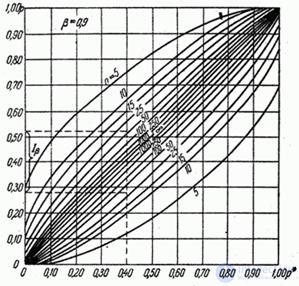
Fig. 14.5.2.

With a given The curves limiting the "confidence region" are determined by the equations:

; (14.5.12)

(14.5.13)

Where - the number of occurrences of the event:

.

Solving equation (14.5.12) for , you can find the lower bound “Trust area”; similarly from (14.5.13) you can find .

In order not to solve these equations anew each time, it is convenient to pre-tabulate (or present graphically) solutions for several typical values ​​of confidence probability. . For example, in the book of I. V. Dunin-Barkovsky and N. V. Smirnov, "Theory of Probability and Mathematical Statistics in Engineering" there are tables and for and . From the same book borrowed graph pic. 14.5.2.

Example 3. Find the confidence limits and for the probability of an event, if in 50 experiments its frequency was . Confidence probability .

Decision. By building (see dashed line in Fig. 14.5.2) for and we find: ; .

Пользуясь методом доверительных интервалов, можно приближенно решить и другой важный для практики вопрос: каково должно быть число опытов для того, чтобы с доверительной вероятностью 3 ожидать, что ошибка от замены вероятности частотой не превзойдет заданного значения?

При решении подобных задач удобнее не пользоваться непосредственно графиками типа рис. 14.5.2, а перестроить их, представив доверительные границы как функции от числа опытов .

Пример 4. Проведено 25 опытов, в которых событие произошло 12 раз. Найти ориентировочно число опытов , которое понадобится для того, чтобы с вероятностью ошибка от замены вероятности частотой не превзошла 20%.

Decision. Определяем предельно допустимую ошибку:

.

Using the curves in fig. 14.5.2, we will construct a new graph: on the abscissa axis we postpone the number of experiments , on the ordinate axis - the confidence limits for the probability (Fig. 14.5.3).

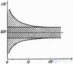
Fig. 14.5.3.

The average straight line parallel to the x-axis corresponds to the observed event frequency .Above and below the straight line are drawn curves. and depicting lower and upper confidence limits depending on .The area between the curves, which determines the confidence interval, is shaded. In the immediate vicinity of a straight double-hatching, a narrower area of ​​20% permissible error is shown. From fig.14.5.3 it is seen that the error falls to the permissible value when the number of experiments is about 100

Note that after performing the required number of experiments, a new verification of the accuracy of determining the probability by frequency may be needed, since in the general case a different frequency value will be obtained that differs from that observed in previous experiments. In this case, it may turn out that the number of experiments is still not enough to ensure the required accuracy, and it will have to be slightly increased. However, the first approximation obtained by the method described above can serve as an indicative preliminary planning of a series of experiments in terms of the time required for them, money costs, etc.

In practice, sometimes you have to meet with a peculiar problem of determining the confidence interval for the probability of an event when the frequency obtained from experience is zero. Such a task is usually associated with experiments in which the probability of the event of interest to us is very small (or, conversely, very high - then the probability of the opposite event is small).

Let, for example, tests of some product on the reliability of work. As a result of testing, the product did not fail once. It is required to find the maximum possible probability of failure.

We set this task in a general form. Produced independent experiments, none of which event Did not happen. Confidence level set ; требуется построить доверительный интервал для вероятности события , точнее - найти его верхнюю границу так как нижняя , естественно, равна нулю.

Поставленная задача является частным случаем общей задачи о доверительном интервале для вероятности, но ввиду своих особенностей заслуживает отдельного рассмотрения. Прежде всего, приближенный метод построения доверительного интервала (на основе замены закона распределения частоты нормальным), изложенный в начале данного , здесь неприменим, так как вероятность очень мала. Точный метод построения доверительного интервала на основе биномиального распределения в данном случае применим, но может быть существенно упрощен.

We will argue as follows. As a result опытов наблюдено событие , состоящее в том, что не появилось ни разу. Требуется найти максимальное значение , которое «совместимо» с наблюденным в опыте событием , если считать «несовместимыми» с те значения , для которых вероятность события меньше, чем .

Очевидно, для любой вероятности события вероятность наблюденного события equals

.

Полагая , получим уравнение для :

, (14.5.14)

from where

. (14.5.15)

Пример 5. Вероятность самопроизвольного срабатывания взрывателя при падении снаряда с высоты неизвестна, но предположительно весьма мала. Произведено 100 опытов, в каждом из которых снаряд роняли с высоты , но ни в одном опыте взрыватель не сработал. Определить верхнюю границу 90%-го доверительного интервала для вероятности .

Decision. По формуле (14.5.15)

,

;

; .

Рассмотрим еще одну задачу, связанную с предыдущей. Event с малой вероятностью не наблюдалось в серии из опытов ни разу. Задана доверительная вероятность . Каково должно быть число опытов для того, чтобы верхняя доверительная граница для вероятности события была равна заданному значению ?

Решение сразу получается из формулы (14.5.14):

. (14.5.16)

Пример 6. Сколько раз нужно убедиться в безотказной работе изделия для того, чтобы с гарантией 95% утверждать, что в практическом применении оно будет отказывать не более чем в 5% всех случаев?

Decision. По формуле (14.5.16) при , we have:

.

Округляя в большую сторону, получим:

.

Имея в виду ориентировочный характер всех расчетов подобного рода, можно предложить вместо формул (14.5.15) и (14.5.16) более простые приближенные формулы. Их можно получить, предполагая, что число появлений события at опытах распределено по закону Пуассона с математическим ожиданием . Это предположение приближенно справедливо в случае, когда вероятность очень мала (см. гл. 5. 5.9). Then

,

и вместо формулы (14.5.15) получим:

, (14.5.17)

а вместо формулы (14.5.16)

. (14.5.18)

Example 7. Find an approximate value for the conditions of example 5.

Decision. By the formula (14.5.14) we have:

,

i.e. the same result, which is obtained by the exact formula in Example 5.

Example 8. Find an approximate value for the conditions of example 6.

Decision. By the formula (14.5.18) we have:

.

Rounding up in a big way, we find that it differs little from the result obtained in Example 6.