Lecture
Let there be a space of elementary events U, a field of events is built on it, and for each event A from this field the probability P (A) is determined. To each elementary event g i from U we associate several numbers: ξ i1 , ξ i2 , ξ i3 , ... ξ ik or vector ξ i . We require that for any x j (-∞ <x j <+ ∞), j = 1, 2 ... k, the set A be those g for which ξ j <x j (j = 1, 2, ... k) belonged to the event field, i.e. for it the probability P {ξ 1 <x 1 , ξ 2 <x 2 , ... ξ k <x k } = P (A) = F (x 1 , x 2 , ... x k ) is defined. Then ξ is called a multidimensional random variable , or a random vector , and F (x 1 , x 2 , ... x k ) is its distribution function .
Examples:
one . The coordinates of a molecule located in a vessel with a gas (x, y, z) or its velocity components (Vx, Vy, Vz) can be viewed as three-dimensional random variables.
2 In the task "about meeting" the time of arrival of one participant (x 1 ) and another (x 2 ), if the conditions of their arrival are known (say, any moment during a given hour), a pair of numbers x 1 , x 2 can be considered as a two-dimensional random variable
3 The result of an experiment consisting in measuring the current through a discharge tube at ten different voltages applied to a tube can be considered as a ten-dimensional random variable.
Properties of the multidimensional distribution function:
one . F (x 1 , x 2 , ... -∞ ... x k ) = 0;
2 F (x 1 , x 2 , ... x k-1 , ∞) = F (x 1 , x 2 , ... x k-1 ), i.e. if one of the arguments takes the value ∞, then the dimension of the random variable is reduced by 1;
3 F (x 1 , x 2 , ... x k ) is a non decreasing function of any argument.
Multidimensional random variables can be continuous , i.e. take any values in a certain region of k-dimensional space (for example, the above-mentioned components of the velocity of a molecule). Their F (x 1 , x 2 , ... x k ) continuous function of all arguments. For them, the k-dimensional distribution density p (x 1 , x 2 , ... x k ), which is the derivative of the distribution function, is determined.
 (7.1)
(7.1)
The probability that a random vector will take a value lying in the region V of the c-dimensional space is equal to the integral over this region of the c-dimensional density of the distribution.
The integral over all variables from - ∞ to + ∞ of k-dimensional distribution density is 1.
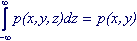
The integral over one variable from - ∞ to + ∞ of the k-dimensional distribution density is equal to the distribution density of the (k-1) -dimensional random variable.
For example:
 (7.2)
(7.2)
Multidimensional random variables can be discrete , i.e. Each component of a random vector can take only a finite or countable set of defined values.
For example, consider an experiment on throwing two bones at the same time, with each elementary event we associate two numbers (z 1 , z 2 ), where z 1 is the number of points on the first bone, z 2 is the sum of points on two bones. Then (z 1 , z 2 ) is a two-dimensional random variable, since the probability p (x i , x k ) of intersection of events is known, consisting in that z 1 takes the value x i , and z 2 - x k . For discrete random variables, the distribution law is given by the probabilities of all possible combinations of their values. For a two-dimensional value with a small number of possible values, it is convenient to present this in the form of a table, where at the intersection of the column z 1 and the line z 2 there is a probability p (z 1 , z 2 )
Table 7.1 The distribution law of the two-dimensional value z 1 , z 2
| z 2 \ z 1 | one | 2 | 3 | four | five | 6 | p (z 2 ) |
| 2 | 1/36 | 0 | 0 | 0 | 0 | 0 | 1/36 |
| 3 | 1/36 | 1/36 | 0 | 0 | 0 | 0 | 1/18 |
| four | 1/36 | 1/36 | 1/36 | 0 | 0 | 0 | 1/12 |
| five | 1/36 | 1/36 | 1/36 | 1/36 | 0 | 0 | 1/19 |
| 6 | 1/36 | 1/36 | 1/36 | 1/36 | 1/36 | 0 | 5/36 |
| 7 | 1/36 | 1/36 | 1/36 | 1/36 | 1/36 | 1/36 | 1/6 |
| eight | 0 | 1/36 | 1/36 | 1/36 | 1/36 | 1/36 | 5/36 |
| 9 | 0 | 0 | 1/36 | 1/36 | 1/36 | 1/36 | 1/9 |
| ten | 0 | 0 | 0 | 1/36 | 1/36 | 1/36 | 1/12 |
| eleven | 0 | 0 | 0 | 0 | 1/36 | 1/36 | 1/18 |
| 12 | 0 | 0 | 0 | 0 | 0 | 1/36 | 1/36 |
| p (z 1 ) | 1/6 | 1/6 | 1/6 | 1/6 | 1/6 | 1/6 |
Summing up all the values of р (z 1 , z 2 ) along each line, we get the probabilities of certain values of z 2 , i.e. distribution law of one-dimensional value z 2 . Similarly, the sum over the columns will give the distribution law of the one-dimensional quantity z 1 . The sum of all numbers in the table should be equal to 1.
The expectation of a multidimensional random variable is a vector, whose components are the expectation of each individual component of a random vector.
M (z 1 , z 2 , ... z k ) = (Mz 1 , Mz 2 , ... Mz k ). Mz i are calculated as a sum or integral as well as for one-dimensional random variables. (see section 6)
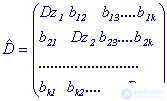
The variance of a multidimensional random variable is described by a covariance matrix  .
.
This is a table of numbers of dimension K × K for a K-dimensional quantity, in which the diagonal contains the variances of the corresponding one-dimensional quantities calculated in the usual way, and the ij-th element is b ij - the covariance coefficient of the i-th and j-th component of the random vector.
 (7.3)
(7.3)
The coefficient of covariance of random variables z i , z j , sometimes denoted as cov (z i , z ji ), is the mathematical expectation of the product of the deviations of each of these values from its expectation:
b ij = cov (z i , z j ) = M [(z i - Mz i ) (z j - Mz j )] (7.4)
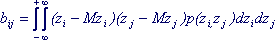
To calculate the covariance coefficient, it is necessary to know the distribution law of a two-dimensional random variable (z i , z j ). Then for continuous values:
 (7.5)
(7.5)
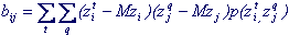
for discrete quantities:
 (7.6)
(7.6)
Here the summation is carried out over all t values that are taken by z i and all q values that are taken by z j .
Transforming (7.4), we obtain a more convenient formula for calculating the coefficient of covariance
b ij = cov (z i , z j ) = M (z i × z j ) - Mz i × Mz j (7.7)
Calculate the characteristics of a two-dimensional value presented in table 7.7
Мz 1 = 1/6 × (1 + 2 + 3 + 4 + 5 + 6) = 3.5
Мz 2 = 2/36 + 3/18 + 4/12 + 5/9 + 30/36 + 7/6 + 40/36 + 9/9 + 10/12 + 11/18 + 12/36 = 7, t .
M (z 1 , z 2 ) = (3.5, 7)
Dz 1 = 1/6 × (1 + 4 + 9 + 16 + 25 + 36) - 3.52 = 3.417
Dz 2 = 4/36 + 9/18 + 16/12 + 25/9 + 36 × (5/36) + 49/6 + 64 × (5/36) + 81/9 + 100/12 + 121/18 + 144/36 - 49 = 5.833
M (z 1 z 2 ) = 1/36 × (1 × 2 + 1 × 3 + 1 × 4 + 1 × 5 + 1 × 6 + 1 × 7 + 2 × 3 + 2 × 4 + 2 × 5 + 2 × 6 + 2 × 7 + 2 × 8 + 3 × 4 + 3 × 5 + 3 × 6 + 3 × 7 + 3 × 8 + 3 × 9 + 4 × 5 + 4 × 6 + 4 × 7 + 4 × 8 + 4 × 9 + 4 × 10 + 5 × 6 + 5 × 7 + 5 × 8 + 5 × 9 + 5 × 10 + 5 × 11 + 6 × 7 + 6 × 8 + 6 × 9 + 6 × 10 + 6 × 11 + 6 × 12) - 3.5 × 7 = 2.917,
those. covariance matrix is:
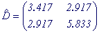 (7.7)
(7.7)
The following concept is often used: the correlation coefficient r ij is the coefficient of covariance divided by the root of the product of the variances of the ith and jth components of a random vector
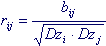 (7.8)
(7.8)
The correlation coefficient r ij may be positive or negative, but never exceeds in absolute value 1.
The components of a multidimensional random variable are called independent if the multidimensional distribution function, multidimensional distribution density, the probability of a certain set of values decay into the product of the corresponding one-dimensional functions or probabilities:
F (x 1 , x 2 , ... x k ) = F (x 1 ) × F (x 2 ) ... × F (x k );
p (x 1 , x 2 , ... x k ) = p (x 1 ) × p (x 2 ) ... × p (x k ); (7.9)
p (x t i , x q j , ... x r k ) = p (x t i ) × p (x q j ) ... × p (x r k );
Conditions (7.9), as well as the conditions arising from them and the definition of conditional probability, which must be satisfied in the entire domain of existence of values of random variables:
p (x i / x j ) = p (x i ), p (x t i / x q j ) = p (x t i ) (7.10)
- signs of independence of random variables
The components z 1 , z 2 of the two-dimensional quantity presented in table 7.7 are not independent, since p (1,4) = Р {z 1 = 1, z 2 = 4} = 1/36,
P {z 1 = 1} = 1/6,
P {z 2 = 4} = 1/12 (condition 7.9 is violated);
p (1/10) = Р {z 1 = 1 / z 2 = 10} = 0,
P {z 1 = 1} = 1/6 (condition 7.10 is violated);
For independent random variables:
The coefficients of covariance and correlation are 0 , therefore, the covariance matrix is diagonal
<p "=" "> b ij = cov (z i , z j ) = r ij = 0The mathematical expectation of the product of independent random variables is equal to the product of mathematical expectations .
<p "=" "> M (z i × z j ) = Mz i × Mz jThe variance of the sum of independent random variables is equal to the sum of their variances.
<p "=" "> D (z i + z j ) = D (z i ) + D (z j )The concept of a random function (random process)
If an elementary event is not matched with a set of numbers (random vector), as in Section 7, but a function of some parameter t - f (t) and the distribution function F t (x) = P {f (t) <x} is defined for each value of t , f (t) is called a random function or a random process . Figuratively speaking, this is an "infinite-dimensional random variable."
If F t (x) does not depend on t, the process is called stationary . The numerical characteristics of a random process (mathematical expectation and variance) for a fixed t are determined in the same way as for an ordinary random variable if the distribution density p t (x) or p t (x i ) is known (if f takes a discrete series of values). For a stationary process, these characteristics are independent of t.
For a stationary process, it is fashionable to calculate statistical characteristics using another method, by averaging over a parameter:
Expected value
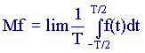 (7.11)
Dispersion
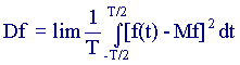 (7.12)
If both methods of calculating numerical characteristics give the same result, the process is called ergodic.
An analogue of the covariance matrix, which characterizes the relationship between components of a random vector, for a random process is the autocorrelation function G (τ), which shows how quickly the values of the random function can change with a parameter change.
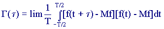 (7.13)

Comments
To leave a comment
Probability theory. Mathematical Statistics and Stochastic Analysis
Terms: Probability theory. Mathematical Statistics and Stochastic Analysis