5.4. Distribution density

Let there be a continuous random variable with distribution function which we assume is continuous and differentiable. Calculate the probability of hitting this random variable on the area from before :

,

those. the increment of the distribution function in this area. Consider the ratio of this probability to the length of the segment, i.e. average probability per unit length in this area, and we will approximate to zero. In the limit, we obtain the derivative of the distribution function:

. (5.4.1)

We introduce the notation:

. (5.4.2)

Function - the derivative of the distribution function - characterizes, as it were, the density with which the values ​​of a random variable at a given point are distributed. This function is called the distribution density (otherwise - "probability density") of a continuous random variable. .

The terms “distribution density”, “probability density” become especially vivid when using the mechanical interpretation of a distribution; in this interpretation the function literally characterizes the density of mass distribution along the abscissa axis (the so-called "linear density"). The curve depicting the density distribution of a random variable is called the distribution curve (Fig. 5.4.1).

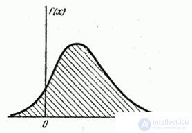
Fig. 5.4.1.

Distribution density, as well as the distribution function, is one of the forms of the distribution law. In contrast to the distribution function, this form is not universal: it exists only for continuous random variables.

Consider a continuous random variable with distribution density and elementary plot adjacent to the point (Fig. 5.4.2). Probability of hitting a random variable on this elementary segment (up to infinitesimal higher order) is equal . Magnitude called the element of probability. Geometrically, this is the area of ​​an elementary rectangle based on a segment (Fig. 5.4.2).

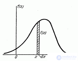
Fig. 5.4.2.

Express the probability of hitting the value on the segment from before (Figure 5.4.3) through the distribution density. Obviously, it is equal to the sum of the elements of probability throughout this segment, i.e. integral:

(5.4.3)

*) Since the probability of any single value of a continuous random variable is zero, we can consider here a segment , not including the left end, i.e. discarding the equal sign in .

Geometrically probability of hitting the value on the plot equal to the area of ​​the distribution curve based on this area (Fig. 5.4.3.).

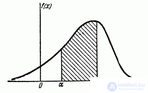
Fig. 5.4.3.

The formula (5.4.2.) Expresses the distribution density through the distribution function. Let us set the inverse problem: to express the distribution function in terms of density. By definition

,

whence by the formula (5.4.3) we have:

. (5.4.4)

Geometrically is nothing but the area of ​​the distribution curve, lying to the left of the point (Fig. 5.4.4).

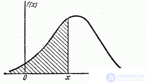
Fig. 5.4.4.

We indicate the main properties of the density distribution.

1. The density of distribution is a non-negative function:

.

This property directly follows from the fact that the distribution function there is a non-decreasing function.

2. The integral in the infinite limits of the distribution density is equal to one:

.

This follows from formula (5.4.4) and from the fact that .

Geometrically, the basic properties of the distribution density mean that:

1) the entire distribution curve does not lie below the abscissa axis;

2) the total area bounded by the distribution curve and the abscissa axis is one.

Let us find out the dimension of the main characteristics of a random variable — the distribution function and the distribution density. Distribution function , like any probability, there is a dimensionless quantity. Distribution density , as can be seen from the formula (5.4.1), is inverse to the dimension of the random variable.

Example 1. The distribution function of a continuous random variable X is given by

a) Find the coefficient a.

b) Find the density of distribution .

c) Find the probability of hitting the value on a site from 0,25 to 0,5.

Decision. a) Since the distribution function of the magnitude continuous then when from where .

b) distribution density expressed by the formula

c) According to the formula (5.3.1) we have:

.

Example 2. Random variable subject to the distribution law with a density of:

at

at or .

a) Find the coefficient a.

b) Build a graph of distribution density .

c) Find the distribution function and build her schedule.

d) Find the probability of hitting the value. on a plot from 0 to .

Decision. a) To determine the coefficient a, we use the property of the density of distribution:

,

from where .

b) density chart presented in fig. 5.4.5.

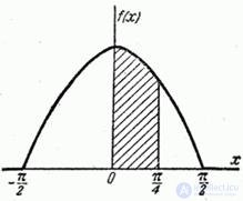
Fig. 5.4.5.

c) According to the formula (5.4.4), we obtain the expression of the distribution function:

Function graph shown in fig. 5.4.6.

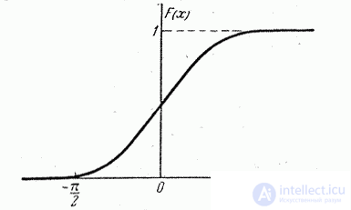
Fig. 5.4.6.

g) According to the formula (5.3.1) we have:

.

The same result, but in a somewhat more complicated way, can be obtained by the formula (5.4.3).

Example 3. The distribution density of a random variable given by the formula:

.

a) Build a density graph .

b) Find the probability that the quantity gets to the site (-1, +1).

Decision. a) The density graph is given in fig. 5.4.7.

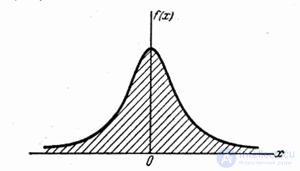
Fig. 5.4.7.

b) According to the formula (5.4.3) we have:

.