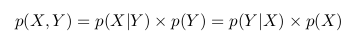
Lecture

Let's consider the following example. Take a coin and throw it 3 times. With the same probability we can get the following results (O - Eagle, P - Tails): LLC, OOR, ORO, ORR, ROO, ROR, PPO, PPP.
We can calculate how many eagles fell in each case and how many shifts were heads-tails, tails-heads:

We can consider the number of eagles and the number of changes as two random variables. Then the probability table will have the following form:

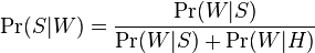
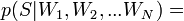
Now we can see the Bayes formula in action.
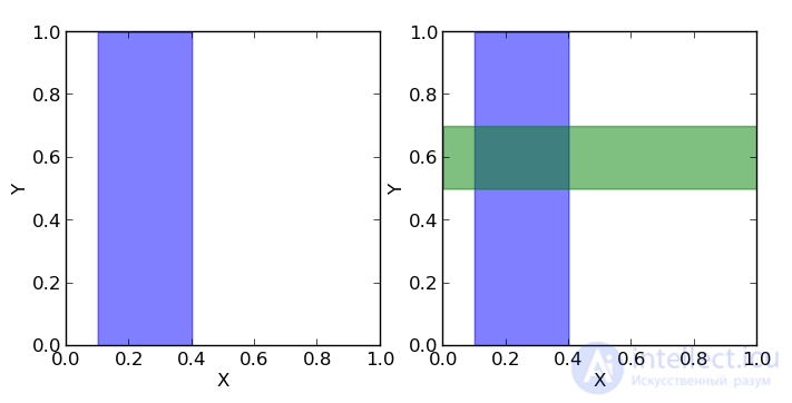
But before we draw an analogy with the square, which we considered earlier.
You can see that p (1O) is the sum of the third column (the “blue area” of the square) and is equal to the sum of all cell values in this column: p (1O) = 2/8 + 1/8 = 3/8
p (1С) is the sum of the third row (the “green area” of the square) and, similarly, is equal to the sum of all cell values in this row p (1С) = 2/8 + 2/8 = 4/8
The probability that we got one eagle and one shift is equal to the intersection of these areas (that is, the value in the cage of the intersection of the third column and the third row) p (1C, 1O) = 2/8
Then, following the formulas described above, we can calculate the probability of getting one shift, if we got one eagle in three throws:
p (1С | 1О) = p (1С, 1О) / p (1О) = (2/8) / (3/8) = 2/3
or the probability of getting one eagle, if we got one shift:
p (1О | 1С) = p (1С, 1О) / p (1С) = (2/8) / (4/8) = 1/2
If we calculate the probability of getting one shift in the presence of one eagle p (1О | 1С) through the Bayes formula, we get:
p (1О | 1С) = p (1С | 1О) * p (1О) / p (1С) = (2/3) * (3/8) / (4/8) = 1/2
What we got higher.
But what practical value does the above example have?
The fact is that when we analyze real data, we are usually interested in some parameter of this data (for example, mean, variance, etc.). Then we can draw the following analogy with the above table of probabilities: let the rows be our experimental data (we denote them Data), and the columns the possible values of the parameter of interest to us this data (we denote it  ). Then we are interested in the probability of obtaining a certain value of the parameter based on the available data.
  .
.
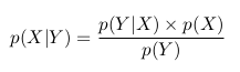
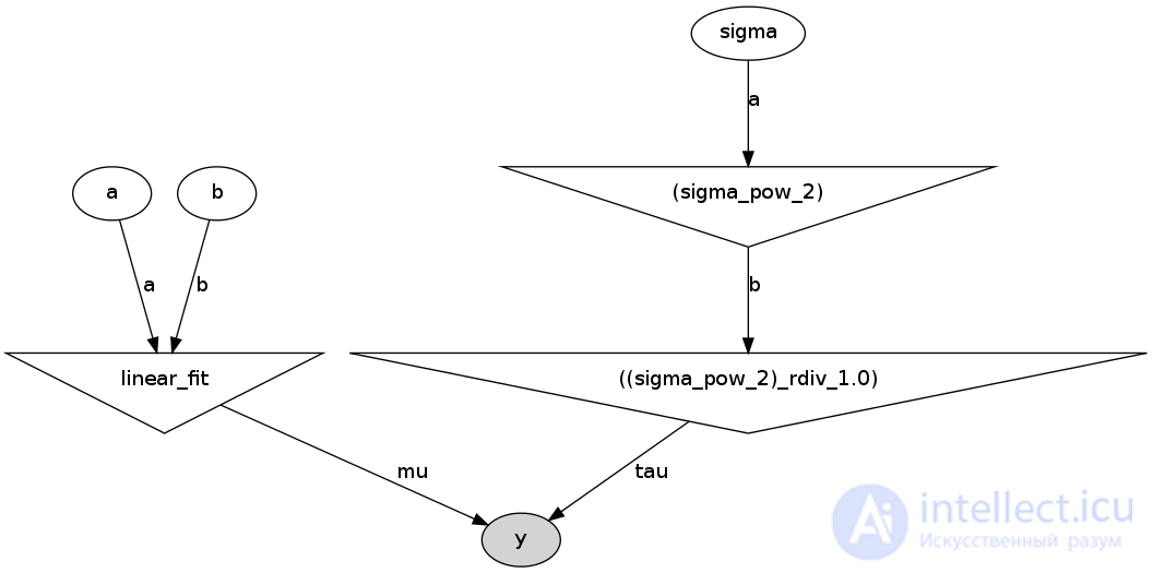
We can apply Baeys formula and write the following:
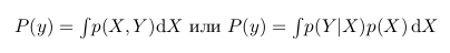
And remembering the formula with the integral, we can write the following:

That is, in fact, as a result of our analysis, we have the probability as a function of a parameter. Now we can, for example, maximize this function and find the most probable parameter value, calculate the variance and average value of the parameter, calculate the boundaries of the segment within which the parameter of interest lies with a probability of 95%, etc.
Probability called a posteriori probability. And in order to calculate it we need to have
 - the likelihood function and
  - a priori probability.
The likelihood function is determined by our model. That is, we create a data collection model that depends on the parameter we are interested in. For example, we want to interpolate data using the straight line y = a * x + b (thus, we assume that all data have a linear relationship with Gaussian noise superimposed on it with known dispersion). Then a and b are our parameters, and we want to know their most probable values, and the likelihood function is Gauss with an average, given by a straight line equation, and a given dispersion.
A priori probability includes the information that we know before the analysis. For example, we know for sure that the straight line should have a positive slope, or that the value at the point of intersection with the x axis should be positive - all this and not only we can incorporate it into our analysis.
As you can see, the denominator fraction is an integral (or in the case when the parameters can take only certain discrete values, the sum) of the numerator over all possible values of the parameter. In practice, this means that the denominator is a constant and serves to normalize the a posteriori probability (that is, the a posteriori probability integral is equal to unity).
This post is a logical continuation of my first post about Bayesian methods, which can be found here.
I would like to talk in detail about how to carry out the analysis in practice.
As I already mentioned, the most popular tool used for Bayesian analysis is the R language with JAGS and / or BUGS packages. For an ordinary user, the difference in packages is in cross-platform JAGS (first-hand experience has made sure there is a conflict between Ubuntu and BUGS), and also that you can create your own functions and distributions in JAGS (however, infrequently, if ever, arises). By the way, an excellent and convenient IDE for R is, for example, RStudio.
But in this post I will write about an alternative to R - Python with the pymc module.
As a convenient IDE for Python, I can offer spyder.
I prefer Python because, firstly, I see no reason to learn such a not too common language like R, just to count some kind of problem related to statistics. Secondly, Python with its modules, from my point of view, is not inferior to R in simplicity, clarity and functionality.
I propose to solve a simple problem of finding the coefficients of linear data dependence. A similar problem of parameter optimization is quite common in various fields of knowledge, so I would say that it is very revealing. In the end, we will be able to compare the result of the Bayesian analysis and the least squares method
First of all, we need to install Python (for those who have not yet done so). I did not use Python 3.3, but with 2.7 everything works fine.
Then you need to install all the necessary modules for Python: numpy, Matplotlib.
If desired, you can also install additional modules: scipy, pyTables, pydot, IPython and nose.
All of these settings (except for Python itself) are easier to do through setuptools.
And now you can install the actual pymc (you can also install it via setuptools).
A detailed guide on pymc can be found here.
We have data obtained during a hypothetical experiment, which linearly depend on a certain quantity x. Data arrives with noise whose dispersion is unknown. It is necessary to find the coefficients of linear dependence.
First we import the modules that we have installed and which we will need:
import numpy import pymc
Then we need to get our hypothetical linear data.
To do this, we determine how many points we want to have (in this case, 20), they are evenly distributed on the interval [0, 10], and set the real coefficients of a linear relationship. Next, we impose on the data Gaussian noise:
#Generate data with noise number_points = 20 true_coefficients = [10.4, 5.5] x = numpy.linspace(0, 10, number_points) noise = numpy.random.normal(size = number_points) data = true_coefficients[0]*x + true_coefficients[1] + noise
So, we have the data, and now we need to think about how we want to conduct an analysis.
First, we know (or assume) that our gaussian noise means that our likelihood function will be gaussian. It has two parameters: mean and variance. Since the noise average is zero, the mean for the likelihood function will be set by the model value (and the model is linear, so there are two parameters). While the variance is unknown to us, therefore, it will be another parameter.
As a result, we have three parameters and a Gaussian likelihood function.
We do not know anything about the values of the parameters; therefore, a priori we assume them to be uniformly distributed with arbitrary boundaries (these boundaries can be moved as far as desired).
When specifying an a priori distribution, we must specify a label by which we will learn about the a posteriori values of the parameters (the first argument), as well as indicate the boundaries of the distribution (the second and third arguments). All of the above arguments are required (there are additional arguments that can be found in the documentation).
sigma = pymc.Uniform('sigma', 0., 100.) a = pymc.Uniform('a', 0., 20.) b = pymc.Uniform('b', 0., 20.)
Now we need to set our model. In pymc there are two of the most commonly used classes: deterministic and stochastic. If, given the input data, you can uniquely determine the value (s) that the model (s) returns, then this is a deterministic model. In our case, given the coefficients of a linear relationship for any point, we can uniquely determine the result, respectively, this is a deterministic model:
@pymc.deterministic(plot=False) def linear_fit(a=a, b=b, x=x): return a*x + b
Finally, we define a likelihood function, in which the mean is the value of the model, sigma is a parameter with a given prior distribution, and data is our experimental data:
y = pymc.Normal('y', mu=linear_fit, tau=1.0/sigma**2, value=data, observed=True)
So, the whole model.py file looks like this:
import numpy import pymc #Generate data with noise number_points = 20 true_coefficients = [10.4, 5.5] x = numpy.linspace(0, 10, number_points) noise = numpy.random.normal(size = number_points) data = true_coefficients[0]*x + true_coefficients[1] + noise #PRIORs: #as sigma is unknown then we define it as a parameter: sigma = pymc.Uniform('sigma', 0., 100.) #fitting the line y = a*x+b, hence the coefficient are parameters: a = pymc.Uniform('a', 0., 20.) b = pymc.Uniform('b', 0., 20.) #define the model: if a, b and x are given the return value is determined, hence the model is deterministic: @pymc.deterministic(plot=False) def linear_fit(a=a, b=b, x=x): return a*x + b #LIKELIHOOD #normal likelihood with observed data (with noise), model value and sigma y = pymc.Normal('y', mu=linear_fit, tau=1.0/sigma**2, value=data, observed=True)
Now I propose to make a small theoretical digression and discuss what pymc does after all.
From the point of view of mathematicians, we need to solve the following problem:
p (a, b, sigma | Data) = p (Data | a, b, sigma) * p (a, b, sigma) / p (Data)
Because a, b and sigma are independent, then we can rewrite the equation as follows:
p (a, b, sigma | Data) = p (Data | a, b, sigma) * p (a) * p (b) * p (sigma) / p (Data)
On paper, the task looks very simple, but when we solve it numerically (we must also think that we want to solve any problem of this class numerically, and not only with certain types of probabilities), then difficulties arise.
p (Data) is, as discussed in my previous post, a constant.
p (Data | a, b, sigma) is definitely given to us (that is, with known a, b and sigma, we can uniquely calculate the probabilities for our available data)
a here, instead of p (a), p (b) and p (sigma), we, in fact, have only pseudo-random variable generators distributed according to the law we specified.
How to get a posteriori distribution from all this? That's right, generate (sample) a, b and sigma, and then read p (Data | a, b, sigma). As a result, we get a chain of values, which is a sample of the posterior distribution. But this raises the question of how we can do this sample correctly. If our a posteriori distribution has several modes ("hills"), then how can we generate a sample covering all the modes. That is, the task is how to effectively make a sample that would “cover” the entire distribution in the least amount of iterations. There are several algorithms for this, the most used of which are MCMC (Markov chain Monte Carlo). The Markov chain is a sequence of random events in which each element depends on the previous one, but does not depend on the previous one. I will not describe the algorithm itself (this may be the topic of a separate post), but just note that pymc implements this algorithm and as a result gives the Markov chain, which is a sample of the a posteriori distribution. Generally speaking, if we do not want the chain to be Markov, then we just need to “thin down” it, i.e. take, for example, every second element.
So, we create a second file, let's call it run_model.py, in which we will generate a Markov chain. The model.py and run_model.py files must be in the same folder, otherwise the code should be added to the run_model.py file:
from sys import path path.append("путь/к/папке/с/файлом/model.py/")
First we import some modules that will be useful to us:
from numpy import polyfit from matplotlib.pyplot import figure, plot, show, legend import pymc import model
polyfit implements the least squares method — we will compare the Bayesian analysis with it.
figure, plot, show, legend are needed in order to build a final schedule.
model is, in fact, our model.
Then we create the MCMC object and run the sample:
D = pymc.MCMC(model, db = 'pickle') D.sample(iter = 10000, burn = 1000)
D.sample takes two arguments (in fact, you can specify more) - the number of iterations and burn-in (let's call it the “warm-up period”). The warm-up period is the number of first iterations that are clipped. The fact is that MCMC initially depends on the starting point (this is a property), so we need to cut off this period of dependence.
This completes our analysis.
Now we have an object D, in which the sample is located, and which has various methods (functions) allowing to calculate the parameters of this sample (mean, most probable value, variance, etc.).
In order to compare the results, we do the analysis of the method of least squares:
chisq_result = polyfit(model.x, model.data, 1)
Now we print all the results:
print "\n\nResult of chi-square result: a= %f, b= %f" % (chisq_result[0], chisq_result[1]) print "\nResult of Bayesian analysis: a= %f, b= %f" % (Davalue, Dbvalue) print "\nThe real coefficients are: a= %f, b= %f\n" %(model.true_coefficients[0], model.true_coefficients[1])
We build standard pymc graphics:
pymc.Matplot.plot(D)
And finally, we build our final schedule:
figure() plot(model.x, model.data, marker='+', linestyle='') plot(model.x, Davalue * model.x + Dbvalue, color='g', label='Bayes') plot(model.x, chisq_result[0] * model.x + chisq_result[1], color='r', label='Chi-squared') plot(model.x, model.true_coefficients[0] * model.x + model.true_coefficients[1], color='k', label='Data') legend() show()
Here is the full content of the run_model.py file:
from numpy import polyfit from matplotlib.pyplot import figure, plot, show, legend import pymc import model #Define MCMC: D = pymc.MCMC(model, db = 'pickle') #Sample MCMC: 10000 iterations, burn-in period is 1000 D.sample(iter = 10000, burn = 1000) #compute chi-squared fitting for comparison: chisq_result = polyfit(model.x, model.data, 1) #print the results: print "\n\nResult of chi-square result: a= %f, b= %f" % (chisq_result[0], chisq_result[1]) print "\nResult of Bayesian analysis: a= %f, b= %f" % (Davalue, Dbvalue) print "\nThe real coefficients are: a= %f, b= %f\n" %(model.true_coefficients[0], model.true_coefficients[1]) #plot graphs from MCMC: pymc.Matplot.plot(D) #plot noised data, true line and two fitted lines (bayes and chi-squared): figure() plot(model.x, model.data, marker='+', linestyle='') plot(model.x, Davalue * model.x + Dbvalue, color='g', label='Bayes') plot(model.x, chisq_result[0] * model.x + chisq_result[1], color='r', label='Chi-squared') plot(model.x, model.true_coefficients[0] * model.x + model.true_coefficients[1], color='k', label='Data') legend() show()
In the terminal we see the following answer:
Result of chi-square result: a = 10.321533, b = 6.307100
Result of Bayesian analysis: a = 10.366272, b = 6.068982
The real coefficients are: a = 10.400000, b = 5.500000
I note that since we are dealing with a random process, the values that you see in yourself may differ from the above (except for the last line).
And in the folder with the file run_model.py we will see the following graphics.
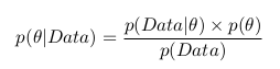
For parameter a:
For parameter b:

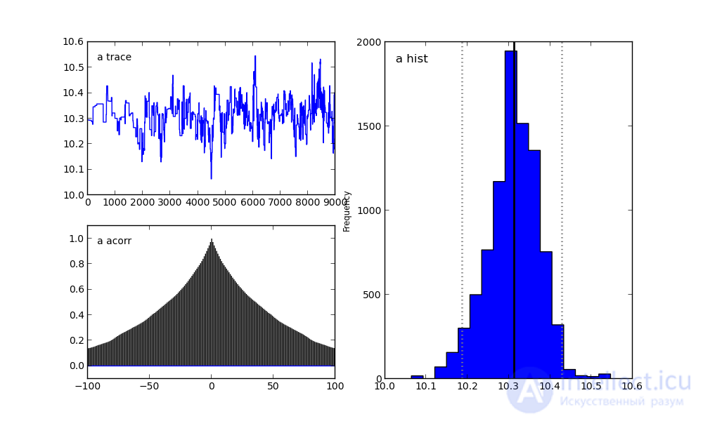
For the sigma parameter:
On the right, we see a histogram of the posterior distribution, and the two pictures on the left belong to the Markov chain.
I will not focus on them now. Let me just say that the bottom graph is the autocorrelation graph (you can read more here). It gives an idea of the convergence of MCMC.
And the top graph shows the sample trace. That is, it shows how the sample took place over time. The average of this trace is the average of the sample (compare the vertical axis in this graph with the horizontal axis in the histogram on the right).
In conclusion, I will talk about one more interesting option.
If you still put the pydot module and include the following line in the run_model.py file:
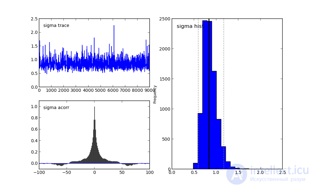
pymc.graph.dag(D).write_png('dag.png')
He will create the following image in the folder with the file run_model.py:
This is a direct acyclic graph representing our model. White ellipses show stochastic nodes (these are a, b and sigma), triangles are deterministic nodes, and a darkened ellipse includes our pseudo-experimental data.
That is, we see that the values a and b come into our model (linear_fit), which itself is a deterministic node, and then go to the likelihood function y. Sigma is first set by the stochastic node, but since the parameter in the likelihood function is not sigma, but tau = 1 / sigma ^ 2, the stochastic value sigma is first squared (the upper triangle on the right), and then it is considered tau. And tau already enters the likelihood function, as well as our generated data.
I think that this graph is very useful both for explaining the model and for self-checking of logic.
models.
Bayesian spam filtering is a spam filtering method based on the use of a naive Bayes classifier based on the use of the Bayes theorem.
The first known mail filtering program using the Bayesian classifier was Jason Rennie’s iFile program, released in 1996. The program used mail sorting by folders [1] . The first academic publication on naive Bayes spam filtering appeared in 1998 [2] . Shortly after this publication, work was started on creating commercial spam filters [ source not specified 906 days ] . However, in 2002, Paul Graham was able to significantly reduce the number of false positives to such an extent that the Bayesian filter could be used as the only spam filter [3] [4] [5] .
Modifications of the basic approach have been developed in many research papers and implemented in software products [6] . Many modern mail clients do Bayesian spam filtering. Users can also install individual mail filtering programs. Mail server filters such as DSPAM, SpamAssassin, SpamBayes, SpamProbe, Bogofilter, CRM114 use Bayesian spam filtering methods [5] . The e-mail server software either includes filters in its delivery, or provides an API for connecting external modules.
When training a filter for each word encountered in letters, its “weight” is calculated and saved - an estimate of the probability that a letter with this word is spam. In the simplest case, the frequency is used as an estimate: “appearances in spam / appearances of everything”. In more complex cases, pre-processing of the text is possible: reduction of words to the initial form, removal of official words, calculation of the “weight” for whole phrases, transliteration, and so on.
When checking a newly arrived letter, the probability of “spamming” is calculated using the above formula for a variety of hypotheses. In this case, “hypotheses” are words, and for each word “accuracy of the hypothesis”  - the share of the word in the letter, and "the dependence of the event on the hypothesis
  - previously calculated "weight" of the word. That is, the “weight” of the letter in this case is the averaged “weight” of all its words.
The assignment of a letter to “spam” or “non-spam” is made according to whether its “weight” exceeds a certain level specified by the user (usually 60-80% is taken). After making a decision on the letter in the database, the “weights” are updated for the words included in it.
Mail Bayes filters are based on Bayes theorem. The Bayes theorem is used several times in the context of spam: for the first time, to calculate the probability that a message is spam, knowing that the given word appears in this message; the second time, to calculate the probability that the message is spam, taking into account all its words (or their corresponding subsets); sometimes for the third time when there are messages with rare words.
Let's assume that the suspect message contains the word "Replica". Most people who are used to receiving an email know that this message is likely to be spam, or more precisely an offer to sell fake watches of famous brands. A spam detection program, however, does not “know” such facts, all it can do is calculate probabilities.
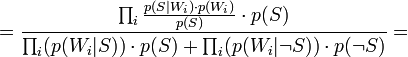
The formula used by the software to determine this is derived from the Bayes theorem and the total probability formula:

Where:
 - the conditional probability that the message is spam, provided that the word "Replica" is in it;
 - the total probability that an arbitrary message is spam;
 - the conditional probability that the word “replica” appears in messages if they are spam;
 - the total probability that an arbitrary message is not spam (i.e., “ham”);
 - the conditional probability that the word “replica” appears in messages if they are “ham”.
Recent statistical studies [7] have shown that today the probability of any message being spam is at least 80%:  .
.
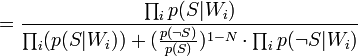
However, most Bayesian spam detection programs suggest that there are no prior preferences for the message to be “spam” rather than “ham”, and it assumes that both cases have equal probability of 50%:  .
.
The filters that use this hypothesis are referred to as “no prejudice” filters. This means that they have no prejudice regarding incoming email. This assumption allows us to simplify the general formula to:
Value  called “spamming” words
  while the number used in the formula above is approximately equal to the relative frequency of messages containing the word in messages identified as spam during the training phase, that is:
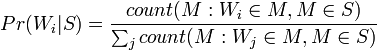
Similar approximately equal to the relative frequency of messages containing the word in messages identified as “ham” during the training phase.
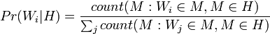
In order for these approximations to make sense, the set of training messages must be large and representative enough. It is also desirable that the training message set matches the 50% hypothesis of a redistribution between spam and ham, that is, that the spam and ham message sets are the same size.
Of course, determining whether a message is “spam” or “ham” based solely on the presence of only one specific word is error-prone, which is why Bayesian spam filters try to look at several words and combine their spamming to determine the overall probability that the message is spam
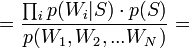
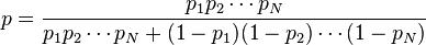
Software spam filters built on the principles of a naive Bayes classifier make a “naive” assumption that events corresponding to the presence of a word in an email or message are independent of each other. This simplification is generally incorrect for natural languages such as English, where the probability of detecting an adjective increases if there is, for example, a noun. Based on this “naive” assumption, to solve the problem of classifying messages only into 2 classes:  (spam) and
  ("Ham", that is, not spam) from the Bayes theorem, we can derive the following formula for estimating the probability of "spaminess" of an entire message containing the words
 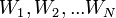 :
:
 [by Bayes theorem]
 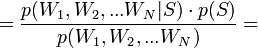 [because
  - are supposed to be independent]
 [by Bayes theorem]
 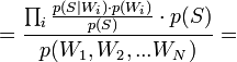 [по формуле полной вероятности]

Таким образом, предполагая 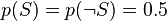 , имеем:
Where:
 — вероятность, что сообщение, содержащее слова
  — спам;
 — условная вероятность
  того, что сообщение — спам, при условии, что оно содержит первое слово (к примеру «replica»);
 — условная вероятность
  того, что сообщение — спам, при условии, что оно содержит второе слово (к примеру «watches»);
 — условная вероятность
  того, что сообщение — спам, при условии, что оно содержит N ое слово (к примеру «home»).
(Demonstration: [8] )
Результат p обычно сравнивают с некоторым порогом, например,  , чтобы решить, является ли сообщение спамом или нет. Если p ниже чем порог, сообщение рассматривают как вероятный «ham», иначе его рассматривают как вероятный спам.
Она возникает в случае, если слово никогда не встречалось во время фазы обучения: и числитель, и знаменатель равны нулю, и в общей формуле, и в формуле спамовости.
В целом, слова, с которыми программа столкнулась только несколько раз во время фазы обучения, не являются репрезентативными (набор данных в выборке мал для того, чтобы сделать надёжный вывод о свойстве такого слова). Простое решение состоит в том, чтобы игнорировать такие ненадёжные слова.
«Нейтральные» слова такие, как, «the», «a», «some», или «is» (в английском языке), или их эквиваленты на других языках, могут быть проигнорированы. Вообще говоря, некоторые байесовские фильтры просто игнорируют все слова, у которых спамовость около 0.5, так как в этом случае получается качественно лучшее решение. Учитываются только те слова, спамовость которых около 0.0 (отличительный признак законных сообщений — «ham»), или рядом с 1.0 (отличительный признаки спама). Метод отсева может быть настроен например так, чтобы держать только те десять слов в исследованном сообщении, у которых есть самое большое absolute value |0.5 − Pr |.
Некоторые программные продукты принимают во внимание тот факт, что определённое слово появляется несколько раз в проверяемом сообщении [9] , другие не делают.
Некоторые программные продукты используют словосочетания — patterns (последовательности слов) вместо изолированных слов естественных языков [10] . Например, с «контекстным окном» из четырех слов, они вычисляют спамовость словосочетания «Виагра, хорошо для», вместо того, чтобы вычислить спамовости отдельных слов «Виагры», «хорошо», и «для». Этот метод более чувствителен к контексту и устраняет байесовский шум лучше, за счет большей базы данных.
Кроме «наивного» байесовского подхода есть и другие способы скомбинировать—объединить отдельные вероятности для различных слов. Эти методы отличаются от «наивного» метода предположениями, которые они делают о статистических свойствах входных данных. Две различные гипотезы приводят к радикально различным формулам для совокупности (объединения) отдельных вероятностей.
Например, для проверки предположения о совокупности отдельных вероятностей, логарифм произведения которых, с точностью до константы подчиняетсяраспределению хи-квадрат с 2 N степенями свободы, можно было использовать формулу:

где C −1 is the inverse of the chi-square function.
Отдельные вероятности могут быть объединены также методами марковской дискриминации.
Данный метод прост (алгоритмы элементарны), удобен (позволяет обходиться без «черных списков» и подобных искусственных приемов), эффективен (после обучения на достаточно большой выборке отсекает до 95—97 % спама, и в случае любых ошибок его можно дообучать). В общем, есть все показания для его повсеместного использования, что и имеет место на практике — на его основе построены практически все современные спам-фильтры.
Впрочем, у метода есть и принципиальный недостаток: он базируется на предположении , что одни слова чаще встречаются в спаме, а другие — в обычных письмах , и неэффективен, если данное предположение неверно. Впрочем, как показывает практика, такой спам даже человек не в состоянии определить «на глаз» — только прочтя письмо и поняв его смысл. Существует метод Байесова отравления ( англ. ), позволяющий добавить много лишнего текста, иногда тщательно подобранного, чтобы «обмануть» фильтр.
Еще один не принципиальный недостаток, связанный с реализацией — метод работает только с текстом. Зная об этом ограничении, спамеры стали вкладывать рекламную информацию в картинку. Текст же в письме либо отсутствует, либо не несёт смысла. Против этого приходится пользоваться либо средствами распознавания текста («дорогая» процедура, применяется только при крайней необходимости), либо старыми методами фильтрации — «черные списки» и регулярные выражения (так как такие письма часто имеют стереотипную форму).

Comments
To leave a comment
Probability theory. Mathematical Statistics and Stochastic Analysis
Terms: Probability theory. Mathematical Statistics and Stochastic Analysis