6.3. The probability of hitting a random variable in a given area. Normal distribution function

The probability of hitting a random variable, subordinate to the normal law, on a given area. Normal distribution function

In many problems associated with normally distributed random variables, it is necessary to determine the probability of a random variable falling. subject to normal law with parameters on the plot from before . To calculate this probability, we use the general formula

, (6.3.1)

Where - size distribution function .

Find the distribution function random variable distributed according to normal law with parameters . Distribution density equals:

. (6.3.2)

From here we find the distribution function

. (6.3.3)

We make in the integral (6.3.3) a change of variable

and bring it to mind:

(6.3.4)

The integral (6.3.4) is not expressed in terms of elementary functions, but it can be calculated through a special function expressing a definite integral of the expression or (the so-called probability integral) for which the tables are compiled. There are many types of such functions, for example:

;

etc. Which of these functions to use is a matter of taste. We will choose as such a function

. (6.3.5)

It is easy to see that this function is nothing but a distribution function for a normally distributed random variable with parameters .

Let's call the function normal distribution function. The appendix (Table 1) contains tables of function values. .

Express the distribution function (6.3.3) values with parameters and through the normal distribution function . Obviously

. (6.3.6)

Now we find the probability of hitting a random variable. on the plot from before . According to the formula (6.3.1)

. (6.3.7)

Thus, we have expressed the probability that a random variable will hit the section. distributed according to the normal law with any parameters through the standard distribution function corresponding to the simplest normal law with parameters 0,1. Note that the function arguments in the formula (6.3.7) have a very simple meaning: there is a distance from the right end of the plot to the center of dispersion, expressed in standard deviations; - the same distance for the left end of the section, and this distance is considered positive if the end is located to the right of the center of dispersion, and negative if it is to the left.

Like any distribution function, the function has properties:

one. .

2 .

3 - non-decreasing function.

In addition, from the symmetry of the normal distribution with parameters relative to the origin it follows that

. (6.3.8)

Using this property, strictly speaking, it would be possible to limit the function tables only positive values ​​of the argument, but to avoid unnecessary operation (subtraction from one), the values ​​in table 1 of the annex are given for both positive and negative arguments.

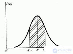
Fig. 6.3.1.

In practice, the problem of calculating the probability of a normally distributed random variable in a region symmetrical about the center of dispersion is often encountered. . Consider this length (fig. 6.3.1). We calculate the probability of hitting this area by the formula (6.3.7):

. (6.3.9)

Given the property (6.3.8) of the function and giving the left side of the formula (6.3.9) a more compact form, we obtain the formula for the probability of a random variable falling on the area symmetric about the center of dispersion according to the normal law:

. (6.3.10)

We solve the following problem. Set aside from the center of dispersion consecutive lengths (Fig. 6.3.2) and calculate the probability of hitting a random variable in each of them. Since the curve of the normal law is symmetric, it is enough to postpone such segments only in one direction.

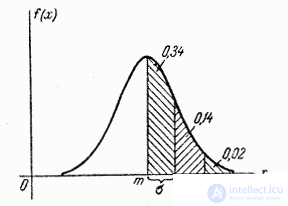
Fig. 6.3.2.

By the formula (6.3.7) we find:

(6.3.11)

As can be seen from these data, the probabilities of hitting each of the following segments (fifth, sixth, etc.) with an accuracy of up to 0.001 are equal to zero.

Rounding the probabilities of hitting the segments to 0.01 (up to 1%), we get three numbers that are easy to remember:

0.34; 0.14; 0.02.

The sum of these three values ​​is 0.5. This means that for a normally distributed random variable, all the dispersions (up to fractions of a percent) fit into the area .

This allows, knowing the mean square deviation and the mathematical expectation of a random variable, to roughly indicate the interval of its practically possible values. This method of estimating the range of possible values ​​of a random variable is known in mathematical statistics as the “three sigma rule”. The approximate method of determining the standard deviation of a random variable also follows from the rule of three sigma: take the maximum practically possible deviation from the average and divide it into three. Of course, this rude reception can be recommended only if there are no other, more accurate ways to determine .

Example 1. Random variable , distributed according to the normal law, is a measurement error of a certain distance. When measuring a systematic error in the direction of overestimation of 1.2 (m); the standard deviation of the measurement error is 0.8 (m). Find the probability that the deviation of the measured value from the true value does not exceed the absolute value of 1.6 (m).

Decision. Measurement error is random subject to normal law with parameters and . It is necessary to find the probability of hitting this quantity from before . By the formula (6.3.7) we have:

.

Using function tables (Appendix, Table 1), we find:

; ,

from where

.

Example 2. Find the same probability as in the previous example, but under the condition that there is no systematic error.

Decision. According to the formula (6.3.10), assuming , we will find:

.

Example 3. The target, having the form of a strip (freeway), whose width is equal to 20 m, is fired in the direction perpendicular to the freeway. Aiming is on the middle line of the highway. The standard deviation in the direction of shooting is m. There is a systematic error in the direction of shooting: 3 m undershoot. Find the probability of hitting the freeway with one shot.

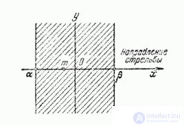
Fig. 6.3.3.

Decision. Select the origin at any point on the middle line of the motorway (Fig. 6.3.3) and direct the x-axis perpendicular to the motorway. Hitting or missing a projectile on a freeway is determined by the value of only one coordinate of the drop point (other coordinate we are indifferent). Random value distributed according to normal law with parameters , . The projectile hit the freeway corresponds to the hit value on the plot from before . Applying the formula (6.3.7), we have:

.

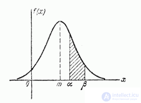
Fig. 6.3.4.

Example 4. There is a random variable , normally distributed, with a dispersion center (fig. 6.3.4) and some section abscissa axis. What should be the standard deviation random variable in order to probability of hitting on the plot reached the maximum?

Decision. We have:

.

Let's differentiate this function :

,

but

.

Applying the rule of differentiation of an integral with respect to a variable entering its limit, we obtain:

.

Similarly

.

To find the extremum, we set:

. (6.3.12)

With this expression vanishes and the probability reaches a minimum. Maximum get from the condition

. (6.3.13)

Equation (6.3.13) can be solved numerically or graphically.