Lecture
In practice, very often random processes occur, occurring in time approximately uniformly and having the form of continuous random oscillations around a certain average value, and neither the average amplitude nor the nature of these oscillations show significant changes over time. Such random processes are called stationary.
As examples of stationary random processes, one can cite: 1) the aircraft oscillations in the steady state of horizontal flight; 2) voltage fluctuations in the electrical lighting network; 3) random noise in the radio; 4) the process of pitching a ship, etc.
Each stationary process can be considered as continuing in time indefinitely; When studying a stationary process, you can choose any time point as a reference point. Investigating the stationary process at any time, we must get the same characteristics. Figuratively speaking, the stationary process "has no beginning or end."
An example of a stationary random process is the change in the height of the center of gravity of an aircraft in a steady state of horizontal flight (Fig. 17.1.1).
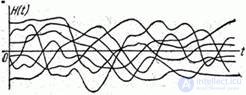
Fig. 17.1.1.
In contrast to stationary stochastic processes, it is possible to point out other, apparently non-stationary, stochastic processes, for example: aircraft vibrations in a dive mode; the process of damped oscillations in the electrical circuit; the process of burning a powder charge in a reactive chamber, etc. The non-stationary process is characterized by the fact that it has a definite tendency of development over time; the characteristics of such a process depend on the origin of the reference, depend on time.
In fig. 17.1.2 depicts a family of implementations of an obviously non-stationary random process — the process of changing the thrust of a jet engine over time.

Fig. 17.1.2.
Note that not all non-stationary random processes are essentially non-stationary throughout their development. There are non-stationary processes that (at known time intervals and with a known approximation) can be taken as stationary.
For example, the process of aiming the crosshair of an aircraft sight to a target is clearly a non-stationary process, if the target passes the sight field of view in a short time with a large and sharply varying angular velocity. In this case, the oscillations of the axis of the sight relative to the target do not have time to be established in a certain stable mode; the process begins and ends without having time to acquire a stationary character. On the contrary, the process of aiming the crosshairs of the sight on a fixed or moving target with a constant angular velocity becomes stationary some time after the start of tracking.
In general, as a rule, a random process in any dynamic system begins with a non-stationary stage - with the so-called "transition process". After the decay of the transition process, the system usually switches to the steady state, and then the random processes occurring in it can be considered stationary.
Stationary random processes are very often found in physical and technical problems. By their nature, these processes are simpler than non-stationary, and are described by simpler characteristics. Linear transformations of stationary random processes are also usually easier than non-stationary ones. In this regard, in practice, the special theory of stationary random processes, or, more precisely, the theory of stationary random functions, is widely used (since the argument of a stationary random function in the general case may not be time). Elements of this theory will be presented in this chapter.
Random function  is called stationary if all its probabilistic characteristics do not depend on
  (more precisely, they do not change with any shift of the arguments on which they depend, along the axis ).
In this elementary presentation of the theory of random functions, we do not at all use such probabilistic characteristics as distribution laws: the only characteristics we use are expectation, variance, and the correlation function. We formulate the definition of a stationary random function in terms of these characteristics.
Since the change in the stationary random function must proceed uniformly over time, it is natural to require that the expectation for the stationary random function be constant:
 . (17.1.1)
Note, however, that this requirement is not essential: we know that from a random function you can always go to centered random function  , for which the mathematical expectation is identically zero and, therefore, satisfies condition (17.1.1). Thus, if a random process is non-stationary only due to a variable mathematical expectation, this does not prevent us from studying it as a stationary process.
The second condition, which, obviously, must be satisfied by a stationary random function, is the condition for the constancy of the variance:
 . (17.1.2)
Let us establish what condition the correlation function of the stationary random function should satisfy. Consider a random function (fig. 17.1.3).
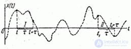
Fig. 17.1.3.
Put in expression 
 and consider
  - the correlation moment of two sections of a random function separated by a time interval
  . Obviously, if a random process is really stationary, this correlation moment should not depend on where exactly on the axis
  we took the plot , and should depend only on the length of this section. For example, for sites
  and
and  in fig. 17.1.3, having the same length , values of correlation function and
  must be the same. In general, the correlation function of a stationary random process should depend not on the position the first argument on the x-axis, but only from the gap between the first and second arguments:
 . (17.1.3)
Consequently, the correlation function of a stationary random process is a function of not two, but only one argument. In some cases, this circumstance greatly simplifies operations on stationary random functions.
We note that condition (17.1.2), which requires constant stationary variance from a stationary random function, is a particular case of condition (17.1.3). Indeed, believing in the formula (17.1.3) 
 we have
 . (17.1.4)
Thus, condition (17.1.3) is the only essential condition that must be satisfied by a stationary random function.
Therefore, in the following, we will understand by a stationary random function such a random function, the correlation function of which does not depend on both of its arguments. and  , but only on the difference between them. In order not to impose special conditions on the expectation, we will consider only centered random functions.
We know that the correlation function of any random function has the symmetry property:
 .
.
Hence for the stationary process, assuming  , we have:
 , (17.1.5)
i.e. correlation function  there is an even function of its argument. Therefore, usually the correlation function is determined only for positive values of the argument (Fig. 17.1.4).

Fig. 17.1.4.
In practice, instead of the correlation function , often use the normalized correlation function
 , (17.1.6)
Where  - constant dispersion of the stationary process. Function
  there is nothing more than a correlation coefficient between the cross sections of a random function separated by an interval on time. It's obvious that
  .
.
As examples, we consider two samples of approximately stationary random processes and construct their characteristics.
Example 1. Random function specified by a set of 12 implementations (Fig. 17.1.5).
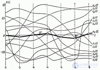
Fig. 17.1.5
a) Find its characteristics  , ,
, ,  and normalized correlation function
  . b) Approximately considering a random function as stationary, find its characteristics.
Decision. Since the random function changes relatively smoothly, it is possible to take sections not very often, for example after 0.4 s. Then the random function will be reduced to a system of seven random variables corresponding to the sections  . By plotting these cross sections on the graph and removing from the graph the values of the random function in these cross sections, we obtain a table (Table 17.1.1).
Table 17.1.1
Implementation number | 0 | 0.4 | 0.8 | 1.2 | 1.6 | 2.0 | 2.4 |
one | 0.64 | 0.74 | 0.62 | 0.59 | 0.35 | -0.09 | 0.39 |
2 | 0.54 | 0.37 | 0.06 | -0.32 | -0,60 | -0.69 | -0.67 |
3 | 0.34 | 0.50 | 0.37 | 0.26 | -0,52 | -0.72 | 0.42 |
four | 0.23 | 0.26 | 0.35 | 0.55 | 0,69 | 0.75 | 0.80 |
five | 0.12 | 0.20 | 0.24 | 0.18 | -0.20 | -0,42 | -0.46 |
6 | -0.16 | -0.12 | -0.15 | 0.05 | 0.29 | 0.43 | 0.63 |
7 | -0,22 | -0.29 | -0.38 | -0.24 | -0.06 | 0.07 | -0.16 |
eight | -0,26 | -0.69 | -0.70 | -0.61 | -0.43 | -0,22 | 0.29 |
9 | -0.50 | -0,60 | -0,68 | -0,62 | -0,68 | -0,56 | -0,54 |
ten | -0.30 | 0.13 | 0.75 | 0.84 | 0.78 | 0.73 | 0.71 |
eleven | -0.69 | -0.40 | 0.08 | 0.16 | 0.12 | 0.18 | 0.33 |
12 | 0.18 | -0.79 | -0,56 | -0,39 | -0,42 | -0,58 | -0,53 |
The table is recommended to fill in the lines, moving all the time along one implementation.
Next, we find estimates for the characteristics of random variables.  . Summing the values by columns and dividing the sum by the number of implementations
  , we will find approximately the dependence of the expectation on time:
| 0 | 0.4 | 0.8 | 1.2 | 1.6 | 2.0 | 2.4 |
| -0,007 | -0,057 | 0,000 | 0.037 | -0,057 | -0,093 | 0.036 |
In the graph of Fig. 17.1.5. The mathematical expectation is shown in bold.
Next, we find estimates for the elements of the correlation matrix: variances and correlation moments. Calculations are most conveniently done as follows. To calculate the statistical variance, the squares of the numbers in the corresponding column are summed; amount divided by ; the square of the corresponding expected value is subtracted from the result. To obtain an unbiased estimate, the result is multiplied by the amendment.  . Correlation moments are estimated similarly. To calculate the statistical moment corresponding to two specified sections, the numbers in the corresponding columns are multiplied; the product is algebraically composed; the amount received is divided by ; the result is the product of the corresponding mathematical expectations; to obtain an unbiased estimate of the correlation moment, the result is multiplied by
  . When performing calculations on a calculating machine or an adding machine, the intermediate results of multiplications are not recorded, but are directly added. The correlation matrix of the system of random variables obtained in this way - it is the table of values of the correlation function
  - given in table 17.1.2.
Table 17.1.2.
| 0 | 0.4 | 0.8 | 1.2 | 1.6 | 2.0 | 2.4 |
0 | 0.1632 | 0.1379 | 0.0795 | 0.0457 | -0,0106 | -0.0642 | -0.0648 |
0.4 | 0.2385 | 0.2029 | 0.1621 | 0.0827 | 0.0229 | 0.0251 | |
0.8 | 0.2356 | 0.2152 | 0.1527 | 0.0982 | 0.0896 | ||
1.2 | 0,2207 | 0.1910 | 0.1491 | 0.1322 | |||
1.6 | 0.2407 | 0.2348 | 0.1711 | ||||
2.0 | 0.2691 | 0.2114 | |||||
2.4 | 0.2878 |
On the main diagonal of the table are estimates of variances:
| 0 | 0.4 | 0.8 | 1.2 | 1.6 | 2.0 | 2.4 |
| 0.1632 | 0.2385 | 0.2356 | 0,2207 | 0.2407 | 0.2691 | 0.278 |
Extracting from these quantities the square roots, we find the dependence of the standard deviation  from time:
| 0 | 0.4 | 0.8 | 1.2 | 1.6 | 2.0 | 2.4 |
| 0.404 | 0.488 | 0.485 | 0.470 | 0,491 | 0.519 | 0.536 |
Sharing the values in table. 17.1.2, to the products of the corresponding standard deviations, we obtain the table of values of the normalized correlation function  (tab. 17.1.3).
Table 17.1.3
| 0 | 0.4 | 0.8 | 1.2 | 1.6 | 2.0 | 2.4 |
0 | one | 0,700 | 0.405 | 0.241 | -0,053 | -0,306 | -0,299 |
0.4 | one | 0.856 | 0.707 | 0.345 | 0.090 | 0.095 | |
0.8 | one | 0.943 | 0.643 | 0.390 | 0.344 | ||
1.2 | one | 0.829 | 0.612 | 0.524 | |||
1.6 | one | 0.923 | 0.650 | ||||
2.0 | one | 0.760 | |||||
2.4 | one |
We analyze the data obtained from the angle of the assumed stationarity of the random function. . Judging directly from the data obtained as a result of processing, it can be concluded that the random function stationary is not: its expectation is not quite constant; the variance also varies somewhat with time; the values of the normalized correlation function along the parallels of the main diagonal are also not quite constant. However, taking into account the very limited number of implementations processed ( ) and in this regard, the presence of a large element of chance in the obtained estimates, these visible deviations from stationarity can hardly be considered significant, especially since they are not of any regular nature. Therefore, an approximate replacement of the function is quite appropriate. stationary. To reduce a function to a stationary, we first of all estimate the time-average estimate for the mathematical expectation
 .
.
Similarly, the mean estimates for the variance are:
 .
.
Extracting the root, we find the averaged estimate of c. K. O .:
 .
.
Let us proceed to the construction of the normalized correlation function of the stationary process, which can replace the random function . For a stationary process, the correlation function (and hence the normalized correlation function) depends only on  ; therefore, with constant the correlation function must be constant. In table 17.1.3 constant correspond: main diagonal (
  ) and parallels of this diagonal (
  ;
;  ;
;  etc.). Averaging the estimates of the normalized correlation function along these parallels of the main diagonal, we obtain the values of the function :
| 0 | 0.4 | 0.8 | 1.2 | 1.6 | 2,0 | 2.4 |
| 1.00 | 0.84 | 0.60 | 0.38 | 0.13 | -0,10 | -0,30 |
Function graph  presented in fig. 17.1.6.
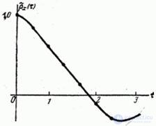
Fig. 17.1.6.
При рассмотрении рис. 17.1.6 обращает на себя внимание наличие для некоторых отрицательных значений корреляционной функции. Это указывает на то, что в структуре случайной функции имеется некоторый элемент периодичности, в связи с чем на расстоянии по времени, равном примерно половине периода основных колебаний, наблюдается отрицательная корреляция между значениями случайной функции: положительным отклонениям от среднего в одном сечении соответствуют отрицательные отклонения через определенный промежуток времени, и наоборот.
Such a character of the correlation function, with a transition to negative values, is very often encountered in practice. Usually in such cases, as the amplitude of the oscillations of the correlation function increases, it decreases and with further increase the correlation function tends to zero.
Example 2. A random function is defined by a set of 12 of its implementations (Fig. 17.1.7). Approximately replacing the function with a stationary one, compare its normalized correlation function with the function of the previous example.
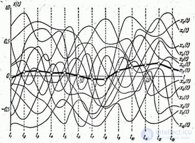
Fig. 17.1.7.
Decision. Так как случайная функция отличается значительно менее плавным ходом по сравнению с функцией предыдущего примера, промежуток между сечениями уже нельзя брать равным 0,4 сек, как в предыдущем примере, а следует взять по крайней мере вдвое меньше (например, 0,2 сек, как на рис. 17.1.7). В результате обработки получаем оценку для нормированной корреляционной функции :
| 0 | 0.2 | 0.4 | 0.6 | 0.8 | 1.0 | 1.2 | 1.4 | 1.6 | 1.8 | 2,0 | 2.2 | 2.4 |
| 1.00 | 0.73 | 0.41 | 0,22 | -0.01 | -0,20 | -0,19 | -0,10 | -0,06 | -0.15 | 0.08 | 0.19 | 0.05 |
Function graph  presented in fig. 17.1.8.
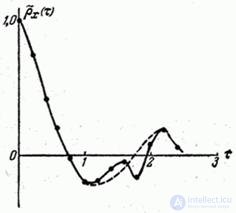
Fig. 17.1.8.
Из сравнения графиков рис. 17.1.8 и 17.1.6 видно, что корреляционная функция, изображенная
in fig. 17.1.8, убывает значительно быстрее. Это и естественно, так как характер изменения функции в примере 1 гораздо более плавный и постепенный, чем в примере 2; в связи с этим корреляция между значениями случайной функции в примере 1 убывает медленнее.
При рассмотрении рис. 17.1.8 бросаются в глаза незакономерные колебания функции для больших значений . Так как при больших значениях точки графика получены осреднением сравнительно очень небольшого числа данных, их нельзя считать надежными. В подобных случаях имеет смысл сгладить корреляционную функцию, как, например, показано пунктиром на рис. 17.1.8.


Comments
To leave a comment
Probability theory. Mathematical Statistics and Stochastic Analysis
Terms: Probability theory. Mathematical Statistics and Stochastic Analysis