Lecture
 . Just like for any other number on the cube.
Violence - the degree (relative measure, quantitative assessment) of the possibility of the occurrence of a certain event. When the grounds for any possible event to occur in reality outweigh the opposing grounds, then this event is called probable , otherwise unlikely or improbable . The preponderance of positive bases over negative ones, and vice versa, can be in varying degrees, as a result of which the probability (and improbability ) is more or less [1] . Therefore, the probability is often assessed at a qualitative level, especially in cases when more or less accurate quantitative assessment is impossible or extremely difficult. There are various gradations of "levels" of probability [2] .
The study of probability from a mathematical point of view is a special discipline - the theory of probability [1] . In probability theory and mathematical statistics, the concept of probability is formalized as a numerical characteristic of an event — a probability measure (or its value) is a measure on a set of events (subsets of a set of elementary events), taking values from  before
  . Value corresponds to a reliable event. An impossible event has a probability of 0 (the reverse is generally not always true). If the probability of occurrence is
  , the probability of its non-occurrence is equal
  . In particular, the probability
  means equal probability of occurrence and non-occurrence of an event.
The classical definition of probability is based on the notion of equal opportunity outcomes. The probability is the ratio of the number of outcomes conducive to this event to the total number of equally possible outcomes. For example, the probability of a “eagle” or “tails” falling out when a coin is accidentally flipped is 1/2 if it is assumed that only these two possibilities take place [3] and they are equally possible. This classical “definition” of probability can be generalized to the case of an infinite number of possible values — for example, if an event can occur with equal probability at any point (the number of points is infinite) of a certain bounded region of space (plane), then the probability that it will occur in some a part of this permissible region is equal to the ratio of the volume (area) of this part to the volume (area) of the area of all possible points.
The empirical "definition" of probability is related to the frequency of the event occurrence, assuming that with a sufficiently large number of tests, the frequency should tend to an objective degree of possibility of this event. In the modern presentation of the theory of probability, probability is defined axiomatically, as a special case of the abstract theory of the measure of set. However, the link between an abstract measure and probability, expressing the degree of possibility of an event, is precisely the frequency of its observation.
Probabilistic description of certain phenomena has become widespread in modern science, in particular in econometrics, of statistical physico-macroscopic (thermodynamic) systems, where even in the case of the classical deterministic description of particle motion, a deterministic description of the entire particle system is not practically possible and expedient. In quantum physics, the processes themselves are of a probabilistic nature.

The need for the concept of probability and research in this direction has been historically associated with gambling, especially with dice. Before the advent of the concept of probability, the combinatorial problems of counting the number of possible outcomes when throwing several dice were formulated, as well as the task of dividing the stakes between players when the game was finished ahead of schedule. The first task when throwing three bones was “solved” in 960 by Bishop Vibold from the city of Cambrai [4] . He counted 56 options. However, this number does not in fact reflect the number of equally probable possibilities, since each of the 56 options can be realized in a different number of ways. In the first half of the 13th century, Richard de Fornival took these aspects into account. Despite the fact that he also has the number 56, but he considers that, for example, “the same number of points on three dice can be obtained in six ways.” Based on his reasoning, it is already possible to establish that the number of equally possible options is 216. In the future, many did not quite correctly solve this problem. For the first time, the number of equally possible outcomes when throwing three bones was calculated by Galileo Galilei, raising the six (the number of options for the loss of one bone) to the power 3 (the number of bones): 6³ = 216. He also compiled a table of the number of ways to obtain different amounts of points.
Problems of the second type at the end of the 15th century formulated and proposed the first (generally speaking erroneous) solution of Luca Pacioli [4] . His decision was to divide the bet in proportion to the games already won. Significant further progress in the early 16th century is associated with the names of Italian scientists Gerolamo Cardano and N. Tartaglia. Cardano gave a correct count of the number of cases when throwing two dice (36). He also for the first time related the number of cases of a number of at least one bone (11) falling out to the total number of outcomes (which corresponds to the classical definition of probability) - 11/36. Similarly, for three bones, he considered, for example, that nine points could be obtained in a number of ways equal to 1/9 of the “whole series” (that is, the total number of equally possible outcomes was 216). Cardano did not formally introduce the notion of probability, but essentially considered the relative number of outcomes, which is essentially equivalent to considering probabilities. It should also be noted that in the embryonic state, Cardano can also find ideas related to the law of large numbers. Regarding the task of dividing the stake, Cardano proposed to take into account the number of remaining games to win. N. Tartaglia also made comments on the decision of Luke and proposed his decision (generally speaking, also erroneous).
The merit of Galileo is also to extend the field of research to the area of observation errors. He first pointed out the inevitability of errors and classified them into systematic and random (such a classification is used now).
The first works on the theory of probability belong to the 17th century. Such as the correspondence of French scientists B. Pascal, P. Fermat (1654) and the Dutch scientist X. Huygens (1657), who gave the earliest known scientific interpretation of probability [5] . In essence, Huygens already operated on the notion of expectation. Swiss mathematician J. Bernoulli, established the law of large numbers for the scheme of independent trials with two outcomes (posthumous, 1713).
In the XVIII century. - early nineteenth century. Probability theory is developed in the works of A. Moivre (England) (1718), P. Laplace (France), C. Gauss (Germany), and S. Poisson (France). Probability theory begins to be applied in the theory of observation errors, which has developed in connection with the needs of geodesy and astronomy, and in the theory of shooting. It should be noted that the law of distribution of errors essentially suggested Laplace first as an exponential dependence on error without taking into account the sign (in 1774), then as an exponential function of the square of the error (in 1778). The latter law is usually referred to as Gaussian distribution or normal distribution. Bernoulli (1778) introduced the principle of the product of probabilities of simultaneous events. Adrien Marie Legendre (1805) developed the least squares method.
In the second half of the XIX century. development of the theory of probability associated with the work of Russian mathematicians P. L. Chebyshev, A. M. Lyapunov and A. A. Markov (senior), as well as work on mathematical statistics A. Quetlet (Belgium) and F. Galton (England) and statistical the physics of L. Boltzmann (in Austria), who created the basis for a significant expansion of the problematics of the theory of probability. The currently most common logical (axiomatic) scheme for constructing the foundations of the theory of probability was developed in 1933 by the Soviet mathematician A. N. Kolmogorov.
The classical "definition" of probability comes from the notion of equal opportunity as an objective property of the phenomena under study. Equality is an indefinable concept and is established from general considerations of symmetry of the phenomena studied. For example, when tossing a coin, it is assumed that by virtue of the assumed coin symmetry, material homogeneity and randomness (impartiality) of tossing, there is no reason to prefer "tails" over "eagle" or vice versa, that is, the falling out of these sides can be considered equally possible (equally likely) .
Along with the notion of equal opportunities in the general case, the classical definition also requires the notion of an elementary event (outcome), favoring or not the event under study A. It is about outcomes, the occurrence of which excludes the possibility of other outcomes. These are incompatible elementary events. For example, when throwing a die, the loss of a specific number excludes the fallout of the remaining numbers.
The classical definition of probability can be formulated as follows:
The probability of a random event A is the ratio of the number n of incompatible equiprobable elementary events that make up event A to the number of all possible elementary events N :

For example, let them throw two bones. The total number of equally possible outcomes (elementary events) is obviously 36 (6 possibilities on each bone). We estimate the probability of dropping 7 points. Obtaining 7 points is possible in the following ways: 1 + 6, 2 + 5, 3 + 4, 4 + 3, 5 + 2, 6 + 1. That is only 6 equally possible outcomes conducive to the event A - getting 7 points. Therefore, the probability will be equal to 6/36 = 1/6. For comparison, the probability of getting 12 points or 2 points is only 1/36 - 6 times less.
Although the classical definition is intuitive and deduced from practice, it can at least not be directly applied if the number of equally possible outcomes is infinite. A striking example of an infinite number of possible outcomes is a bounded geometric region G, for example, on a plane, with an area S. A randomly “tossed” “point” with equal probability can be at any point of this region. The task is to determine the probability of hitting a point in some subdomain g with area s. In this case, generalizing the classical definition, we can come to a geometric definition of the probability of hitting a subdomain  :
:

In view of the equal probability, this probability does not depend on the shape of the region g, it depends only on its area. This definition can naturally be generalized to a space of any dimension, where instead of area to use the concept of "volume". Moreover, this definition leads to the modern axiomatic definition of probability. The concept of volume is generalized to the concept of a measure of an abstract set, to which the requirements that the “volume” has in a geometrical interpretation are presented - first of all, it is non-negativity and additivity.
The classic definition in dealing with complex problems comes up against difficulties of an irresistible nature. In particular, in some cases it may not be possible to identify equally possible cases. Even in the case of a coin, as is well known, there is a clearly not equally probable possibility of falling out of an “edge”, which cannot be estimated from theoretical considerations (one can only say that it is unlikely and that this consideration is more practical). Therefore, at the dawn of the development of probability theory, an alternative “frequency” definition of probability was proposed. Namely, formally, the probability can be defined as the limit of the frequency of observations of event A, assuming uniformity of observations (that is, the same conditions of observation) and their independence from each other:
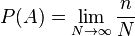
Where  - the number of observations, and
  - number of occurrences
  .
.
Despite the fact that this definition rather indicates a method for estimating an unknown probability - by a large number of homogeneous and independent observations - nevertheless, this definition reflects the content of the notion of probability. Namely, if an event is assigned a certain probability, as an objective measure of its possibility, then this means that under fixed conditions and repeated repetition, we should receive a frequency of its occurrence close to (the closer, the more observations). Actually, this is the original meaning of the concept of probability. The basis is an objectivist view of natural phenomena. Below, we will consider the so-called laws of large numbers, which provide a theoretical basis (within the framework of the modern axiomatic approach outlined below), including for the frequency estimate of probability.
In the modern mathematical approach, the probability is given by Kolmogorov's axioms. It is assumed that some elementary event space is defined.  . Subsets of this space are interpreted as random events . The union (sum) of some subsets (events) is interpreted as an event consisting in the occurrence of at least one of these events. The intersection (product) of subsets (events) is interpreted as an event consisting in the occurrence of all these events. Non-intersecting sets are interpreted as incompatible events (their joint offensive is impossible). Accordingly, an empty set means an impossible event.
Probability ( probability measure ) is a measure (numerical function)  specified on a set of events with the following properties:
 ,
, at
at  then
then 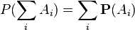 .
. ,
,If the space of elementary events X is finite, then this additivity condition for arbitrary two incompatible events suffices, from which additivity will follow for any finite number of incompatible events. However, in the case of an infinite (countable or uncountable) space of elementary events, this condition is not enough. What is required is the so-called countable or sigma additivity , that is, the fulfillment of the additivity property for any at most than a countable family of pairwise incompatible events. This is necessary to ensure the "continuity" of the probability measure.
The probability measure may not be defined for all subsets of the set . It is supposed to be defined on some sigma-algebra  subsets [6] . These subsets are called measurable in a given probabilistic measure and they are random events. Aggregate
  - that is, the set of elementary events, the sigma-algebra of its subsets, and the probability measure - is called a probability space.
The basic properties of probability are easiest to determine based on the axiomatic definition of probability.
1) the probability of an impossible event (empty set  ) is zero:

Это следует из того, что каждое событие можно представить как сумму этого события и невозможного события, что в силу аддитивности и конечности вероятностной меры означает, что вероятность невозможного события должна быть равна нулю.
2) если событие A «входит» в событие B, то есть  , то есть наступление события A влечёт также наступление события B, то:
Это следует из неотрицательности и аддитивности вероятностной меры, так как событие  , возможно, «содержит» кроме события ещё какие-то другие события, несовместные с .
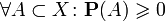
3) вероятность каждого события находится от 0 до 1, то есть удовлетворяет неравенствам:
Первая часть неравенства (неотрицательность) утверждается аксиоматически, а вторая следует из предыдущего свойства с учётом того, что любое событие «входит» в , а для аксиоматически предполагается  .
.
4) вероятность наступления события  , заключающегося в наступлении события при одновременном ненаступлении события , равна:

Это следует из аддитивности вероятности для несовместных событий и из того, что события and являются несовместными по определению, а их сумма равна событию .
5) вероятность события  , противоположного событию , равна:
Это следует из предыдущего свойства, если в качестве множества использовать всё пространство и учесть, что .
6) ( probability addition theorem ) probability of occurrence of at least one of (that is, the sum) of arbitrary (not necessarily incompatible) two events and equals:

This property can be obtained if the union of two arbitrary sets is represented as the union of two disjoint - the first and the difference between the second and the intersection of the original sets:  . Hence, taking into account the additivity of the probability for non-intersecting sets and the formula for the probability of the difference (see property 4) of the sets, we obtain the required property.
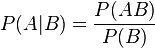
The probability of an event , subject to the occurrence of an event , is called the conditional probability (under this condition) and is denoted by . Наиболее просто вывести формулу определения условной вероятности исходя из классического определения вероятности. Для данных двух событий and рассмотрим следующий набор несовместных событий:
  , которые исчерпывают все возможные варианты исходов (такой набор событий называют полным — см. ниже). Общее количество равновозможных исходов равно . Если событие уже наступило, то равновозможные исходы ограничивается лишь двумя событиями
  , что эквивалентно событию . Пусть количество этих исходов равно
  . Из этих исходов событию благоприятстствуют лишь те, что связаны с событием
  . Количество соответствующих исходов обозначим
  . Тогда согласно классическому определению вероятности вероятность события при условии наступления события будет равна
 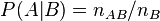 , разделив числитель и знаменатель на общее количество равновозможных исходов и повторно учитывая классическое определение, окончательно получим формулу условной вероятности:
 .
.
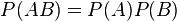
Отсюда следует так называемая теорема умножения вероятностей :
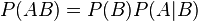 .
.
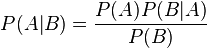
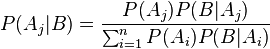
В силу симметрии, аналогично можно показать, что также 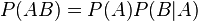 , отсюда следует формула Байеса:
События A и B называются независимыми , если вероятность наступления одного из них не зависит от того, наступили или нет другие события. С учетом понятия условной вероятности это означает, что 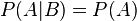 , откуда следует, что для независимых событий выполнено:
В рамках аксиоматического подхода данная формула принимается как определение понятия независимости двух событий. Для произвольной (конечной) совокупности событий  их независимость в совокупности означает, что вероятность их совместного наступления равна произведению их вероятностей:

Выведенная (в рамках классического определения вероятности) выше формула условной вероятности при аксиоматическом определении вероятности является определением условной вероятности. Соответственно, как следствие определений независимых событий и условной вероятности получается равенство условной и безусловной вероятностей события.
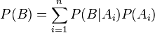
Набор событий  , хотя бы одно из которых обязательно (с единичной вероятностью) наступит в результате испытания, называется полным . Это означает, что набор таких событий исчерпывает все возможные варианты исходов. Формально в рамках аксиоматического подхода это означает, что
  . Если эти события несовместны, то в рамках классического определения это означает, что сумма количеств элементарных событий, благоприятствующих тому или иному событию, равно общему количеству равновозможных исходов.
Пусть имеется полный набор попарно несовместных событий . Тогда для любого события верна следующая формула расчета его вероятности (формула полной вероятности):
Тогда вышеописанную формулу Байеса с учетом полной вероятности можно записать в следующем виде:
Данная формула является основой альтернативного подхода к вероятности — байесовского или субъективного подхода (см. ниже).
Важнейший частный случай применения «вероятности» — вероятность получения в результате испытания или наблюдения того или иного числового значения некоторой измеряемой (наблюдаемой) величины. Предполагается, что до проведения испытания (наблюдения) точное значение этой величины неизвестно, то есть имеется явная неопределенность, связанная обычно (за исключением квантовой физики) с невозможностью учета всех факторов, влияющих на результат. Такие величины называют случайными . В современной теории вероятностей понятие случайной величины формализуется и она определяется как функция «случая» — функция на пространстве элементарных событий. При таком определении наблюдаются не сами элементарные события, а «реализации», конкретные значения случайной величины. Например, при подбрасывании монетки выпадает «решка» или «орел». Если ввести функцию, ставящую в соответствие «решке» — число 1, а «орлу» — 0, то получим случайную величину как функцию указанных исходов. При этом понятие случайной величины обобщается на функции, отображающие пространство элементарных событий в некоторое пространство произвольной природы, соответственно можно ввести понятия случайного вектора, случайного множества и т. д. Однако, обычно под случайной величиной подразумевают именно числовую функцию (величину).
Distracting from the described formalization, the space of elementary events can be understood as the set of possible values of a random variable. The sigma-algebra of subsets are arbitrary intervals on the number axis, their various (countable) unions and intersections. In this case, the probability measure is called the distribution of a random variable. It is enough to specify a probability measure for the intervals of the form  Since an arbitrary interval can be represented as a union or intersection of such intervals. It is assumed that each interval of the above type is associated with a certain probability
 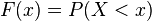 , i.e. some function of possible values
  . Such a function is called an integral, cumulative, or simply a distribution function of a random variable. In the case of differentiability of this function (in this case, the corresponding random variables are called continuous ), also often a more convenient function is introduced analytically — the distribution density — the derivative of the distribution function:
 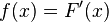 . In the case of discrete random variables, instead of density (it does not exist in this case), you can use the distribution series directly
  - probability
  th value. The corresponding distribution function will be associated with a number of distribution like:
 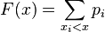 . The probability that a random variable will be in a certain interval
  is defined as the difference of the values of the distribution function at the ends of this interval. Through the density, the distribution is the corresponding integral of the density in a given interval (for a discrete random variable, it is simply the sum of the probabilities of values from this interval).
The distribution of a random variable gives its full characteristic. However, individual characteristics of this distribution are often used. First of all, this is the mathematical expectation of a random variable — the average expected value of a random variable, taking into account the weighting by the probabilities of the occurrence of certain values, and the variance or variation — the average square of the deviation of the random variable from its expectation. In some cases, other characteristics are used, among which asymmetry and kurtosis are important. The described indicators are special cases of the so-called moments of distribution .
There are some standard distribution laws that are often used in practice. First of all, it is the eonormal distribution (Gaussian distribution). It is completely characterized by two parameters - expectation and variance. Its wide use is connected, in particular, with the so-called limit theorems (see below). When testing hypotheses, chi-square distributions, Student's t-distribution, Fisher distribution often occur. In analyzing discrete random variables, the binomial distribution, the Poisson distribution, etc. are also considered. Gamma distribution is also often considered, a special case of which is the exponential distribution, as well as the above Chi-squared distribution. Naturally, the distributions used in practice are not limited to these distributions.
Often in practice, based on a priori considerations, it is assumed that the probability distribution of a given random variable refers to a certain distribution known up to parameters. For example, besides the normal distribution, but with an unknown expectation and variance (these two parameters uniquely determine the entire normal distribution). The task of statistical sciences (mathematical statistics, econometrics, etc.) in this case is to estimate the values of these parameters in the most efficient (accurate) way. There are criteria by which you can establish the degree of "truth" of the relevant assessment methods. Usually, at a minimum, consistency of assessment, unbiasedness and efficiency in a certain class of assessments is required.
In practice, nonparametric methods for estimating distributions are also used.
The group of theorems, usually united under the name “the law of large numbers ” or limit theorems, is of paramount importance in the theory of probability and in its applications. Without resorting to rigorous formulations, it can be said, for example, that under certain weak conditions the average value of independent identically distributed random variables tends to their mathematical expectation with a sufficiently large number of these random variables. If we consider independent observations of the same random variable as a set of random variables, then this means that the average of random observations should tend to the true (unknown) expectation of this random variable. This is the law of large numbers in the form of Chebyshev. This provides a basis for obtaining relevant estimates.
A very special, but very important case is the Bernoulli scheme - independent tests, as a result of which a certain event either occurs or not. It is assumed that in each trial the probability of an event occurring is the same and is equal to (but she is unknown). This scheme can be reduced to the average value if you enter a formal random variable X, which is an indicator of the occurrence of an event: it is equal to 1 when an event occurs and 0 if the event does not occur. For such a random variable, the expectation is also equal to . Then the average value of such a random variable is actually the frequency of the event . According to the above theorem, this average (frequency) should tend to the true expectation of this random variable, that is, to an unknown probability . Thus, with an increase in the number of observations, the frequency of occurrence of an event can be used as a good estimate of the unknown probability. This is the so-called law of large Bernoulli numbers. This law was historically the first law of large numbers. More strictly, it can be argued at least that the probability that the frequency deviates from by some amount  tends to zero for any values . A more general result (the Glivenko – Cantelli theorem) is that the empirical distribution as a whole tends to a true probability distribution with increasing number of observations.
Along with these theorems, there is a so-called central limit theorem, which gives the limit probability distribution for the average, namely, under certain weak conditions, the average value of observations of a random variable with a sufficiently large number of observations have a normal distribution ( regardless of the initial distribution of the random variable itself). For example, this is the case for the average value of independent identically distributed random variables. In particular, this theorem is applicable to the Bernoulli scheme. In general, the number of occurrences of the event A in n tests has a binomial distribution, however, with a sufficiently large number of observations, this distribution, according to the indicated theorem, tends to a normal distribution in this case with a mathematical expectation  and variance
  where - probability of occurrence of event A in each trial. This is stated in the local and integral Muavre-Laplace theorems. This also implies the above conclusion, namely: the average value of the random variable indicator of the event - that is, the frequency of occurrence of the event in the tests - will have in the limit the expectation and variance
  which tends to zero with increasing number of trials. Thus, the frequency tends to the true probability of an event with an increase in the number of independent tests, and we know the frequency distribution with a sufficiently large number of observations.
The basis of the above objective (frequency) approach is the assumption of the presence of objective uncertainty inherent in the studied phenomena. In the alternative Bayesian approach, uncertainty is interpreted subjectively - as a measure of our ignorance. In the framework of the Bayesian approach, probability refers to the degree of confidence in the truth of a judgment — subjective probability.
The idea of the Bayesian approach is to move from a priori knowledge to a posteriori, taking into account the observed phenomena. The essence of the Bayesian approach follows from the Bayes formula described above. Let there be a full set of hypotheses , and from a priori considerations, the probabilities of the validity of these hypotheses are evaluated (the degree of confidence in them). The completeness of a set means that at least one of these hypotheses is true and the sum of a priori probabilities  equal to 1. Also for the event under study from a priori considerations known probabilities
  - probability of occurrence , subject to the validity of the hypothesis . Then, using the Bayes formula, one can determine posterior probabilities
  - that is, the degree of confidence in the hypothesis after the event happened. Actually, the procedure can be repeated taking new probabilities for a priori and again doing the test, thereby iteratively refining the a posteriori probabilities of the hypotheses.
In particular, unlike the basic approach to estimating distributions of random variables, where it is assumed that the values of unknown distribution parameters are estimated based on observations, the Bayesian approach assumes that the parameters are also random variables (in terms of our ignorance of their values). Some possible values of parameters act as hypotheses and certain a priori densities of unknown parameters are assumed to be data.  . The a posteriori distribution serves as an estimate of the unknown parameters. Let some values be obtained from observations studied random variable. Then, for the values of a given sample, assuming the known likelihood is the probability (density) of obtaining a given sample for given values of the parameters
  , using the Bayesian formula (in this case, a continuous analogue of this formula, where density instead of probability takes part, and summation is replaced by integration) we obtain the posterior probability (density)
  parameters for this sample.
Let there be equally likely outcomes. The degree of uncertainty of experience in this situation can be characterized by the number  . This indicator, introduced by the Hartley communication engineer in 1928, describes the information you need to have in order to know which of of equal options exists, that is, to reduce the uncertainty of experience to zero. The simplest way to find out is to ask questions such as “the number of the outcome is less than half N”, if so, you can ask a similar question for one of the halves (depending on the answer to the question), etc. The answer to each such question reduces uncertainty. In total, such questions for the complete removal of uncertainty will need just
  . More formally, the outcome numbers can be represented in binary number system, then Is the number of necessary bits for such a representation, that is, the amount of information in bits, with which you can encode the implementation of equally possible outcomes. In general, the unit of information may be different, so the logarithm can theoretically be used with any base.
In the general case (outcomes are not necessarily equiprobable) the amount of information associated with the implementation of one of outcomes that are probable (assumed  ) is defined as follows (Shannon's formula):
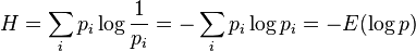
Where  - a sign of mathematical expectation.
Obviously, with equal probability of all outcomes (  ) we get the already known ratio
  . For a continuous random variable in this formula, it is necessary to use instead of probabilities the distribution density function and instead of the sum the corresponding integral.
This value is called information, information quantity, information entropy, etc. It should be noted that such a definition of information abstracts from any information content, content of specific outcomes. Informational quantity is determined only on the basis of probabilities. Magnitude Shannon called entropy due to its similarity with thermodynamic entropy. The last concept was first introduced by Rudolf Clausis in 1865, and Ludwig Boltzmann gave a probabilistic interpretation of entropy in 1877. The entropy of a macroscopic system is a measure of the number of possible microstates for a given macrostate (more specifically, it is proportional to the logarithm of the number of microstates — a statistical weight) or a measure of the “internal disorder” of the macrosystem.
In quantum mechanics, the state of a system (particle) is characterized by a wave function (generally speaking a state vector) —a complex-valued function of “coordinates”, the square of the module of which is interpreted as the probability density of obtaining specified values of “coordinates”. According to modern concepts, the probabilistic definition of a state is complete and the probabilistic nature of quantum physics is not any “hidden” factors - this is due to the nature of the processes themselves. In quantum physics, any interconversions of various particles that are not prohibited by one or another conservation laws are possible. And these interconversions are subject to laws - probabilistic laws. According to modern concepts, it is fundamentally impossible to predict neither the moment of interconversion, nor a specific result. We can only talk about the probabilities of certain transformation processes. Instead of exact classical quantities in quantum physics, only an estimate of the mean values (mathematical expectation) of these quantities is possible, for example, the average lifetime of a particle.
In addition to the question of the likelihood of fact, there may arise, both in the field of law and in the field of moral (with a well-known ethical point of view) the question of how likely it is that this particular fact constitutes a violation of a general law. This question, which serves as the main motive in the religious jurisprudence of Talmud, also in Roman Catholic moral theology (especially from the end of the 16th century) gave rise to very complex systematic constructions and a vast literature, dogmatic and polemical (see Probabilism) [1] .

Comments
To leave a comment
Probability theory. Mathematical Statistics and Stochastic Analysis
Terms: Probability theory. Mathematical Statistics and Stochastic Analysis