Lecture
Introduced in the previous  system characteristic - the distribution function - exists for systems of any random variables, both discontinuous and continuous. The main practical importance are systems of continuous random variables. The distribution of a system of continuous quantities is usually characterized not by a distribution function, but by a distribution density.
Introducing the distribution density for one random variable, we defined it as the limit of the ratio of the probability of hitting a small area to the length of this area with its unlimited decrease. Similarly, we determine the distribution density of a system of two quantities.
Let there be a system of two continuous random variables.  which is interpreted by a random point on the plane
  . Consider a small rectangle on this plane.
  with the parties
  and
and  adjacent to the point with coordinates
  (fig. 8.3.1). The probability of hitting this rectangle by the formula (8.2.2) is equal to

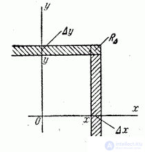
Fig. 8.3.1
Divide the probability of hitting the rectangle. on the area of this rectangle and go to the limit at  and
and  :
:
 (8.3.1)
Suppose the function  not only continuous, but differentiable; then the right side of the formula (8.3.1) is the second mixed partial derivative of the function by
  and
and  . We denote this derivative
  :
:
 (8.3.2)
Function called the distribution density of the system.
Thus, the distribution density of the system is the limit of the ratio of the probability of hitting a small rectangle to the area of this rectangle, when both of its dimensions tend to zero; it can be expressed as the second mixed partial derivative of the distribution function of the system with respect to both arguments.
If we use the "mechanical" interpretation of the distribution of the system as the distribution of a unit mass over the plane function is the mass density distribution at .
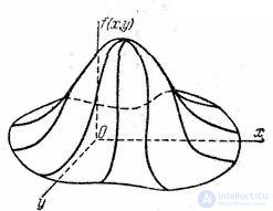
Fig. 8.3.2
Geometrically function can be depicted as a surface (Fig. 8.3.2). This surface is similar to the distribution curve for one random variable and is called the distribution surface.
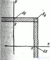
Fig. 8.3.3
If you cross the distribution surface plane parallel to the plane , and project the resulting section on the plane , we get a curve, at each point of which the distribution density is constant. Such curves are called equal density curves. Curves of equal density, obviously, represent the horizontal surface distribution. It is often convenient to set the distribution of a family of curves of equal density.
Considering the density of distribution  for one random variable, we introduced the concept of "probability element"
  . This is the probability of hitting a random variable.
  on the elementary plot
  adjacent to the point . A similar concept of the “probability element” is introduced for a system of two quantities. The element of probability in this case is the expression
 .
.
Obviously, the element of probability is nothing but the probability of falling into an elementary rectangle with sides ,  adjacent to the point (fig. 8.3.3).
This probability is equal to the volume of the elementary parallelepiped bounded above by the surface and based on the elementary rectangle  (fig. 8.3.4).
Using the concept of an element of probability, we derive an expression for the probability of a random point hitting an arbitrary region  . This probability can obviously be obtained by summing (integrating) probability elements over the entire region :
 (8.3.3)
Geometrically probability of hitting the area depicted by the volume of a cylindrical body  bounded above the surface of the distribution and based on the area (fig. 8.3.5).
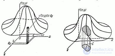
Fig. 8.3.4 Figure 8.3.5
The general formula (8.3.3) implies the formula for the probability of hitting the rectangle  limited by abscissas
  and
and  and ordinates
  and
and  (fig. 8.3.5);
 . (8.3.4)
We use the formula (8.3.4) in order to express the distribution function of the system through density distribution . Distribution function there is a chance of falling into an infinite quadrant; the latter can be considered as a rectangle bounded by abscissas -  and and ordinates - and . By the formula (8.3.4) we have:
 . (8.3.5)
It is easy to verify the following properties of the distribution density of the system:
1. The distribution density of a system is a non-negative function:
 .
.
This is clear from the fact that the distribution density is the limit of the ratio of two non-negative values: the probability of hitting the rectangle and the area of the rectangle — and, therefore, cannot be negative.
2. The double integral in the infinite limits of the distribution density of the system is equal to one:
 (8.3.6)
This is evident from the fact that the integral (8.3.6) is nothing more than the probability of hitting the entire plane. i.e. probability of a reliable event.
Geometrically, this property means that the total volume of the body bounded by the surface distribution and the plane , is equal to one.
Example 1. A system of two random variables subject to the distribution law with density
 .
.
Find distribution function . Determine the probability of hitting a random point. in square (fig. 8.3.6).
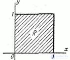
Fig. 8.3.6
Decision. Distribution function we find by the formula (8.3.5).
 .
.
Probability of hitting a rectangle we find by the formula (8.3.4):
 .
.
Example 2. System distribution surface is a straight circular cone, the base of which is a circle of radius centered at the origin. Write an expression for the density of distribution. Determine the probability that a random point will fall into a circle  radius
  (fig. 8.3.7), and
  .
.
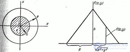
Fig. 8.3.7 Figure 8.3.8
Decision. The expression of the density of the distribution inside the circle we find from fig. 8.3.8:
 ,
,
Where  - the height of the cone. Magnitude determined so that the volume of the cone was equal to one:
  from where
 ,
,
and
 .
.
Probability of hitting the circle determined by the formula (8.3.4):
 . (8.3.7)
To calculate the integral (8.3.7), it is convenient to go to the polar coordinate system  :
:
 .
.

Comments
To leave a comment
Probability theory. Mathematical Statistics and Stochastic Analysis
Terms: Probability theory. Mathematical Statistics and Stochastic Analysis