10.3. Applications of theorems on numerical characteristics

In this We will demonstrate the application of the apparatus of numerical characteristics to the solution of a number of problems. Some of these tasks have independent theoretical value and will find application in the future. Other tasks are in the nature of examples and are given to illustrate the derived general formulas on a specific digital material.

Task 1. The correlation coefficient of linearly dependent random variables.

Prove that if random variables and linked by linear functional dependence

,

their correlation coefficient is or depending on the sign of the coefficient .

Decision. We have:

,

Where - variance of magnitude .

For the correlation coefficient, we have the expression:

. (10.3.1)

For determining find the variance of the value :

,

.

Substituting in the formula (10.3.1), we have:

.

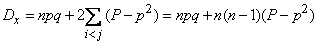
Magnitude equals when positively and when negatively, as it was required to prove.

Task 2. The boundaries of the correlation coefficient.

Prove that for any random variables

.

Decision. Consider a random variable:

,

Where - standard deviations of magnitudes . Determine the variance of the value . According to the formula (10.2.13) we have:

,

or

.

Since the variance of any random variable cannot be negative,

,

or

,

from where

,

and consequently,

,

Q.E.D.

Task 3. Designing a random point on a plane onto an arbitrary line.

Given a random point on a plane with coordinates (fig. 10.3.1). Project this point on the axis drawn through the origin at an angle to the axis . Point projection on axis there is also a random point; her distance from the origin is a random variable. It is required to find the mean and variance .

Fig.10.3.1

Decision. We have:

.

Because there is a linear argument function and then

;

,

Where - variance and correlation moment values .

Turning to the standard deviations, we get:

. (10.3.2)

In the case of uncorrelated random variables (with )

. (10.3.3)

Task 4. Mathematical expectation of the number of occurrences of an event with several experiments.

Produced by experiences, in each of which an event may or may not appear . Probability of occurrence at m experience is . Find the expected number of occurrences of the event.

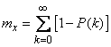
Decision. Consider a discontinuous random variable - the number of occurrences of the event in the entire series of experiments. Obviously

,

Where - the number of occurrences of the event in the first experience

- the number of occurrences of the event in the second experience,

……………………………………………………….

- the number of occurrences of the event in m experience

or shorter

,

Where - the number of occurrences of the event in m experience.

Each of the quantities there is a discontinuous random variable with two possible values: and . Distribution range has the form:

(10.3.4)

Where - probability of non-occurrence at m experience.

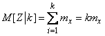
By the theorem of addition of mathematical expectations

, (10.3.5)

Where - expected value .

Calculate the expected value . By the definition of expectation

.

Substituting this expression into formula (10.3.5), we have

, (10.3.6)

that is, the mathematical expectation of the number of occurrences of an event in several experiments is equal to the sum of the probabilities of the event in individual experiments.

In particular, when the conditions of the experiments are the same and

,

the formula (10.3.5) takes the form

. (10.3.7)

Since the theorem of addition of mathematical expectations applies to any random variables, both dependent and independent, formulas (10.3.6) and (10.3.7) are applicable to any experiments, dependent and independent.

The derived theorem is often used in the theory of shooting, when it is required to find the average number of hits for several shots - dependent or independent. The mathematical expectation of the number of hits with several shots is equal to the sum of the probabilities of hit with individual shots.

Task 5. Dispersion of the number of occurrences of an event with several independent experiments.

Produced by independent experiences, in each of which an event may occur , with the probability of occurrence at m experience is . Find the variance and standard deviation of the number of occurrences .

Decision. Consider a random variable - the number of occurrences . Just as in the previous task, let's represent the value as a sum:

,

Where - the number of occurrences of the event in m experience.

By virtue of the independence of experiments, random variables are independent and the dispersion addition theorem is applicable to them:

.

Find the variance of the random variable . From the distribution series (10.3.4) we have:

,

from where

, (10.3.8)

that is, the variance of the number of occurrences of an event with several independent experiments is equal to the sum of the probabilities of the occurrence and non-occurrence of an event in each experiment.

From the formula (10.3.8) we find the standard deviation of the number of occurrences of the event :

. (10.3.9)

With unchanged experimental conditions, when , formulas (10.3.8) and (10.3.9) are simplified and take the form:

(10.3.10)

Task 6. Dispersion of the number of occurrences of the event in dependent experiments.

Produced by dependent experiences in each of which an event may appear with the probability of an event at m experience is . Determine the variance of the number of occurrences of the event.

Decision. In order to solve the problem, we again represent the number of occurrences of the event. as a sum:

, (10.3.11)

Where

Since the experiments are dependent, it is not enough for us to set the probabilities

that event will occur in the first, second, third, etc., experiments. It is also necessary to specify the characteristics of the dependence of the experiments. It turns out that to solve our problem, it is enough to set the probabilities event sharing how in m and so m experience: . Suppose these probabilities are given. Apply to expression (10.3.11) the sum dispersion theorem (formula (10.2.10)):

, (10.3.12)

Where - correlation moment of magnitudes :

.

According to the formula (10.2.19)

. (10.3.13)

Consider a random variable . Obviously it is zero if at least one of the values is equal to zero, i.e. at least in one of the experiments ( m or m) event did not appear. In order to magnitude was equal to one, it is required that in both experiments ( m and m) event appeared. The probability of this is . Consequently,

,

and

.

Substituting this expression into formula (10.3.12), we get:

. (10.3.14)

Formula (10.3.14) and expresses the variance of the number of occurrences of an event in dependent experiments. Let us analyze the structure of this formula. The first term on the right-hand side of the formula represents the variance of the number of occurrences of an event in independent experiments, and the second gives an “correction for dependence”. If the probability equals then this amendment is zero. If the probability more than This means that the conditional probability of an event at experience provided that experience, it appeared more than the simple (unconditional) probability of an event occurring in m experience (between occurrences of an event in m and m experiences there is a positive correlation). If this is the case for any pair of experiments, then the correction term in formula (10.3.14) is positive and the variance of the number of occurrences of the event with dependent experiments is greater than with independent ones.

If the probability less than (between occurrences of an event in m and m experiences there is a negative correlation), then the corresponding term is negative. If this is the case for any pair of experiments, then the variance of the number of occurrences of an event with dependent experiments is less than with independent ones.

Consider a special case when , , ie, the conditions of all experiments are the same. The formula (10.3.14) takes the form:

, (10.3.15)

Where - probability of occurrence immediately in a pair of experiments (no matter what).

In this particular case, two subcases are of particular interest:

1. The event in any of the experiments it entails with certainty his appearance in each of the others. Then , and the formula (10.3.15) takes the form:

.

2. The event in any of the experiments excludes his appearance in each of the others. Then , и формула (10.3.15) принимает вид:

.

Задача 7. Математическое ожидание числа объектов, приведенных в заданное состояние.

На практике часто встречается следующая задача. Имеется некоторая группа, состоящая из объектов, по которым осуществляется какое-то воздействие. Каждый из объектов в результате воздействия может быть приведен в определенное состояние (например, поражен, исправлен, обнаружен, обезврежен и т. п.). Probability that -й объект будет приведен в состояние equal to . Найти математическое ожидание числа объектов, которые в результате воздействия по группе будут приведены в состояние .

Decision. Свяжем с каждым из объектов случайную величину , которая принимает значения or :

Random value - число объектов, приведенных в состояние , - может быть представлена в виде суммы:

.

Отсюда, пользуясь теоремой сложения математических ожиданий, получим:

.

Математическое ожидание каждой из случайных величин известно:

.

Consequently,

, (10.3.16)

т. е. математическое ожидание числа объектов, приведенных в состояние , равно сумме вероятностей перехода в это состояние для каждого из объектов.

Особо подчеркнем, что для справедливости доказанной формулы вовсе не нужно, чтобы объекты переходили в состояние независимо друг от друга. Формула справедлива для любого вида воздействия.

Задача 8. Дисперсия числа объектов, приведенных в заданное состояние.

Если в условиях предыдущей задачи переход каждого из объектов состояние происходит независимо от всех других, то, применяя теорему сложения дисперсий к величине

,

get the variance of the number of objects given in the state :

, . (10.3.17)

If the impact on objects is made so that the transitions to the state for individual objects are dependent, then the variance of the number of objects transferred to the state will be expressed by the formula (see task 6)

, (10.3.18)

Where - the probability that as a result of exposure th and objects will go to state together .

Problem 9. The mathematical expectation of the number of experiments before the th event appears.

A number of independent experiments are carried out, in each of which an event can occur with probability. .Experiments are conducted until the event appears once, after which the experiments are terminated. Determine expected value, variance and c. ko the number of experiments that will be made.

Decision.In Example 3 5.7, the expectation and variance of the number of experiments before the first occurrence of an event were determined. :

, ,

Where - probability of occurrence of an event in one experiment, - probability of non- occurrence .

Consider a random variable - the number of experiences before the event . It can be represented as a sum:

,

Where - the number of experiences before the first occurrence of the event ,

- the number of experiments from the first to the second occurrence of the event (counting the second),

……………………………………………………………………………………………

- the number of experiences from the th to the th occurrence of the event (counting ).

Obviously the magnitude independent; each of them is distributed according to the same law as the first one (the number of experiments before the first occurrence of the event) and has numerical characteristics

, .

Applying the theorems of addition of mathematical expectations and variances, we get:

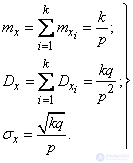(10.3.19)

Task 10. The average expenditure of funds to achieve the desired result.

В предыдущей задаче был рассмотрен случай, когда предпринимается ряд опытов с целью получения вполне определенного результата - появлений события , которое в каждом опыте имеет одну и ту же вероятность. Эта задача является частным случаем другой, когда производится ряд опытов с целью достижения любого результата , вероятность которого с увеличением числа опытов возрастает по любому закону . Предположим, что на каждый опыт расходуется определенное количество средств . Требуется найти математическое ожидание количества средств, которое будет израсходовано.

Decision. Для того чтобы решить задачу, сначала предположим, что число производимых опытов ничем не ограничено, и что они продолжаются и после достижения результата .Then some of these experiences will be superfluous. Let us agree to call the experience “necessary” if it is produced with a result that has not yet been achieved , and “redundant” if it is produced with the result already achieved .

We associate with each ( th) experience a random variable that is zero or one, depending on whether this experience was “necessary” or “redundant”. Set

Consider a random variable - the number of experiments that will have to be made to get the result . Obviously, it can be represented as a sum:

(10.3.20)

Of the quantities on the right-hand side of (10.3.20), the first is nonrandom and is always equal to one (the first experience is always “necessary”). Each of the others is a random variable with possible values. and . Construct a series of distribution of a random variable. . It looks like:

(10.3.21)

Where - probability of achieving the result after experiences.

Indeed, if the result has already been achieved in previous experiments, then (experience is redundant), if not achieved, then (experience is necessary).

Find the expected value . From the distribution series (10.3.21) we have:

.

It is easy to make sure that the same formula will be valid when , because .

Apply to expression (10.3.20) the theorem of addition of mathematical expectations. We get:

or denoting ,

. (10.3.22)

Every experience requires an expense . Multiplying the resulting value on , we define the average cost of funds to achieve the result :

. (10.3.23)

This formula is derived under the assumption that the value of each experience is the same. If this is not the case, then another method can be applied - to present the total expenditure of funds as the sum of the costs of performing individual experiments, which takes two values: , if a experience is “necessary,” and zero if it is “redundant.” The average expense will be presented in the form:

. (10.3.24)

Problem 11. The mathematical expectation of the sum of a random number of random terms.

In a number of practical applications of probability theory one has to meet with sums of random variables, in which the number of terms is unknown in advance, by chance.

Let's set the following task. Random value represents the sum random variables:

, (10.3.25)

and - also a random variable. Suppose that we know the mathematical expectations of all terms:

и что величина не зависит ни от одной из величин .

Требуется найти математическое ожидание величины .

Decision. Число слагаемых в сумме есть дискретная случайная величина. Предположим, что нам известен ее ряд распределения:

Where - вероятность того, что величина took meaning . Зафиксируем значение и найдем при этом условии математическое ожидание величины (условное математическое ожидание):

. (10.3.26)

Теперь применим формулу полного математического ожидания, для чего умножим каждое условное математическое ожидание на вероятность соответствующей гипотезы и сложим:

. (10.3.27)

Особый интерес представляет случай, когда все случайные величины имеют одно и то же математическое ожидание:

.

Тогда формула (10.3.26) принимает вид:

and

. (10.3.28)

Сумма в выражении (10.3.28) представляет собой не что иное, как математическое ожидание величины :

.

From here

, (10.3.29)

т. е. математическое ожидание суммы случайного числа случайных слагаемых с одинаковыми средними значениями (если только число слагаемых не зависит от их значений) равно произведению среднего значения каждого из слагаемых на среднее число слагаемых.

Снова отметим, что полученный результат справедлив как для независимых, так и для зависимых слагаемых лишь бы число слагаемых не зависело от самих слагаемых.

Ниже мы решим ряд конкретных примеров из разных областей практики, на которых продемонстрируем конкретное применение общих методов оперирования с числовыми характеристиками, вытекающих из доказанных теорем, и специфических приемов, связанных с решенными выше общими задачами.

Пример 1. Монета бросается 10 раз. Определить математическое ожидание и среднее квадратическое отклонение числа выпавших гербов.

Decision. По формулам (10.3.7) и (10.3.10) найдем:

; ; .

Пример 2. Производится 5 независимых выстрелов по круглой мишени диаметром 20 см. Прицеливание - по центру мишени, систематическая ошибка отсутствует, рассеивание - круговое, среднее квадратическое отклонение см. Найти математическое ожидание и с. к. о. числа попаданий.

Decision. Вероятность попадания в мишень при одном выстреле вычислим по формуле (9.4.5):

.

Пользуясь формулами (10.3.7) и (10.3.10), получим:

; ; .

Example 3. Airborne attack is carried out, in which 20 type 1 aircraft and 30 type 2 aircraft are involved. Type 1 aircraft are attacked by fighter aircraft. The number of attacks per device is subject to the Poisson law with the parameter . Each attack of a fighter aircraft type 1 is affected with probability .Type 2 aircraft are attacked by anti-aircraft missiles. The number of missiles sent to each device is subject to Poisson’s law with a parameter ; each missile hits a type 2 aircraft with probability . All devices that are part of the raid are attacked and attacked independently of each other. To find:

1) expectation, variance, and c. ko the number of type 1 aircraft affected;

2) expectation, variance, and c. ko the number of type 2 aircraft affected;

3) expectation, variance, and c. ko the numbers of affected aircraft of both types.

Decision. Instead of “the number of attacks” on each device of type 1, we consider “the number of attacking attacks”, also distributed according to the Poisson law, but with a different parameter:

.

The probability of hitting each of the aircraft of type 1 will be equal to the probability that it will have at least one striking attack:

.

The probability of damage to each of the aircraft type 2 will find the same:

.

The mathematical expectation of the number of affected devices of type 1 will be:

.

Dispersion and with. ko this number:

, .

Expectation, number variance and c. ko Type 2 affected devices:

, , .

Mathematical expectation, variance and c. ko total number of affected devices of both types:

, , .

Example 4. Random variables and represent the elementary errors that occur at the input of the device. They have mathematical expectations and dispersions and ; the correlation coefficient of these errors is . The error at the output of the device is connected with errors at the input by the functional dependence:

.

Find the expected value of the error at the output of the device.

Decision.

.

Using the connection between the initial and central moments and formula (10.2.17), we have:

;

;

,

from where

.

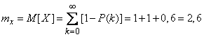
Example 5. An airplane bombing a motorway with a width of 30 m (Fig. 10.3.2). Flight direction is angle with the direction of the motorway. Aiming - on the middle line of the motorway, systematic errors are absent. Dispersion given by the main probable deviations: in the direction of flight m and in the lateral direction m. Find the probability of hitting the highway when dropping a single bomb.

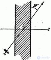
Fig. 10.3.2

Decision. Design a random point of impact on the axis perpendicular to the motorway and apply the formula (10.3.3). It obviously remains fair if we substitute probable deviations instead of the mean-square ones:

.

From here

, .

We will find the probability of hitting the highway by the formula (6.3.10):

.

Note. The method used here for recalculating scattering to other axes is only suitable for calculating the probability of hitting a region in the form of a band; for a rectangle whose sides are turned at an angle to the scattering axes, it is no longer suitable. The probability of hitting each of the lanes whose intersection forms a rectangle can be calculated using this technique, but the probability of hitting the rectangle is no longer equal to the product of the probabilities of hitting the lanes, since these events are dependent.

Example 6. A group of objects is monitored using a radar system for some time; the group consists of four objects; each one in time is found with a probability equal to:

, , , .

Find the expectation of the number of objects that will be detected in time. .

Decision. By the formula (10.3.16) we have:

.

Example 7. A series of events are taken, each of which, if it takes place, brings random net income. normal distributed with average (conventional units). The number of events for a given period of time is random and distributed according to the law.

and does not depend on the income generated by the events. Determine the average expected income for the entire period.

Decision. Based on task 11 of this find the expectation of total income :

,

Where - the average income from one event, - average expected number of events. We have:

,

,

.

Example 8. Device error is expressed by function.

(10.3.30)

Where - the so-called "primary errors", representing a system of random variables (random vector).

Random vector characterized by mathematical expectations

; ;

and correlation matrix:

.

Determine the mean, variance and standard deviation of the instrument error.

Decision. Since the function (10.3.30) is linear, applying formulas (10.2.6) and (10.2.13), we find:

,

,

.

Example 9. To detect the source of a malfunction in a computer, tests are carried out. In each sample, failure is independent of other samples is localized with probability . On average, each sample takes 3 minutes. Find the expectation of the time it takes to isolate the problem.

Decision. Using the result of task 9 given (mathematical increase in the number of experiments to th event occurrence ), believing find the average number of samples

.

These five samples will require an average of

(minutes).

Example 10. Shooting at a fuel tank is performed. The probability of hitting each shot is 0.3. The shots are independent. At the first hit in the reservoir, only the fuel flow appears, at the second hit the fuel is ignited. After the ignition of the fuel, the shooting stops. Find the mathematical expectation of the number of shots fired.

Decision. Using the same formula as in the previous example, we find the mathematical expectation of the number of shots before the 2nd hit:

.

Example 11. The probability of an object being detected by a radar with an increase in the number of review cycles increases according to the law

,

Where - the number of cycles since the beginning of the observation.

Find the mathematical expectation of the number of cycles after which the object will be detected.

Decision. Using the results of task 10 of this section, we obtain:

.

Example 12. In order to perform a specific task of gathering information, several scouts are sent to a given area. Each scout sent to the area of ​​destination with a probability of 0.7. To complete the task, it is sufficient to have three intelligence officers in the area. One scout cannot cope with the task at all, and two scouts perform it with a probability of 0.4. Continuous communication with the area is ensured, and additional scouts are sent only if the task has not yet been completed.

It is required to find the expectation of the number of intelligence officers to be sent.

Decision. Denote - The number of scouts arrived in the area, which was sufficient to complete the task. In task 10 of this the mathematical expectation of the number of experiments was found, which is needed in order to achieve a certain result, the probability of which increases with the increase in the number of experiments according to the law . This expectation is:

.

In our case:

; ; ; ;

.

Expectation value equally:

.

So, in order for the task to be completed, it is necessary that an average of 2.6 scouts arrive in the area.

Now we solve the following problem. How many scouts will on average have to be sent to the area in order for them to arrive on average ?

Let sent scouts. The number of arrived scouts can be represented as

,

where is the random variable takes the value 1 if th scout arrived, and 0 if not arrived. Magnitude is nothing but the sum of a random number of random terms (see Problem 11 of this ). With this in mind, we have:

,

from where

,

but where - probability of arrival of the dispatched scout (in our case ). Magnitude we have just found and equal to 2.6 We have:

.

Example 13. A radar station looks in the area of ​​space in which it is located objects. In one review cycle, it detects each of the objects (independently of the other cycles) with probability . One cycle takes time . How long will it take to objects detect on average ?

Decision. We first find the expectation of the number of objects detected after review cycles. Behind cycles one (any) of the objects is detected with probability

,

and the average number of objects found in cycles, by the expectation addition theorem (see problem 5 of this ) is equal to:

.

Putting

,

get the required number of cycles from the equation

,

deciding which, we find:

,

where does the time required for detection on average objects will be equal to:

.

Example 14. Let us change the conditions of Example 13. Let the radar station monitor the area only until it is detected. objects, after which the observation stops or continues in the new mode. Find the expectation of the time it takes.

In order to solve this problem, it is not enough to ask the probability of detecting one object in one cycle, but you also need to indicate how the probability of objects will be detected at least . The easiest way to calculate this probability, if we assume that objects are detected independently of each other. We make this assumption and solve the problem.

Decision. With independent detections you can monitor objects represent how independent experiences. After cycles, each of the objects is detected with probability

.

Probability that after cycles will be detected at least objects from , we find by the theorem on the repetition of experiments:

.

The average number of cycles, after which will be detected at least objects, determined by the formula (10.3.22):

.

Example 15. On a plane random point with coordination deviates from the required position (origin) under the influence of three independent vector errors , and . Each of the vectors is characterized by two components:

, ,

(fig. 10.3.3). The numerical characteristics of these three vectors are:

, , , , ,

, , , , ,

, , , , .

Fig. 10.3.3

Найти характеристики суммарной ошибки (вектора, отклоняющего точку от начала координат).

Decision. Применяя теоремы сложения математических ожиданий, дисперсий и корреляционных моментов, получим:

,

,

, ,

, ,

,

Where

,

,

,

from where

and

.

Пример 16. Тело, которое имеет форму прямоугольного параллелепипеда с размерами летит в пространстве, беспорядочно вращаясь вокруг центра массы так, что все его ориентации одинаково вероятны. Тело находится в потоке частиц, и среднее число частиц, встречающихся с телом, пропорционально средней площади, которую тело подставляет потоку. Найти математическое ожидание площади проекции тела на плоскость, перпендикулярную направлению его движения.

Decision. Так как все ориентации тела в пространстве одинаково вероятны, то направление плоскости проекций безразлично. Очевидно, площадь проекции тела равна половине суммы проекций всех граней параллелепипеда (так как каждая точка проекции представляет собой проекцию двух точек на поверхности тела). Применяя теорему сложения математических ожиданий и формулу для средней площади проекции плоской фигуры (см. пример 3 10.1), получим:

,

Where - полная площадь поверхности параллелепипеда.

Заметим, что выведенная формула справедлива не только для параллелепипеда, но и для любого выпуклого тела: средняя площадь проекции такого тела при беспорядочном вращении равна одной четверти полной его поверхности. Рекомендуем читателю в качестве упражнения доказать это положение.

Пример 17. На оси абсцисс движется случайным образом точка по следующему закону. В начальный момент она находится в начале координат и начинает двигаться с вероятностью вправо и с вероятностью to the left. Пройдя единичное расстояние, точка с вероятностью продолжает двигаться в том же направлении, а с вероятностью меняет его на противоположное. Пройдя единичное расстояние, точка снова с вероятностью продолжает движение в том направлении, в котором двигалась, а с вероятностью меняет его на противоположное и т. д.

В результате такого случайного блуждания по оси абсцисс точка after шагов займет случайное положение, которое мы обозначим . Требуется найти характеристики случайной величины : математическое ожидание и дисперсию.

Decision. Прежде всего, из соображений симметрии задачи ясно, что . Чтобы найти , представим в виде суммы слагаемых:

, (10.3.31)

Where - расстояние, пройденное точкой на -м шаге, т. е. , если точка двигалась на этом шаге вправо, и , если она двигалась влево.

По теореме о дисперсии суммы (см. формулу (10.2.10)) имеем:

.

It's clear that , так как величина takes values and с одинаковой вероятностью (из тех же соображений симметрии). Найдем корреляционные моменты

.

Начнем со случая , когда величины and стоят рядом в сумме (10.3.31). It's clear that принимает значение with probability и значение with probability . We have:

.

Рассмотрим, далее, случай . В этом случае произведение equally , если оба перемещения - на -м и -м шаге - происходят в одном и том же направлении. Это может произойти двумя способами. Или точка все три шага - -й, th and -й - двигалась в одном и том же направлении, или же она дважды изменила за эти три шага свое направление. Найдем вероятность того, что :

.

Найдем теперь вероятность того, что . Это тоже может произойти двумя способами: или точка изменила свое направление при переводе от -го шага к -му, а при переходе от -го шага к -му сохранила его, или наоборот. We have:

.

Thus, the magnitude имеет два возможных значения and , которые она принимает с вероятностями соответственно and .

Ее математическое ожидание равно:

.

Легко доказать по индукции, что для любого расстояния между шагами в ряду справедливы формулы:

,

,

and therefore

.

Таким образом, корреляционная матрица системы случайных величин будет иметь вид:

.

Random Variance будет равна:

,

или же, производя суммирование элементов, стоящих на одном расстоянии от главной диагонали,

.

Пример 18. Найти асимметрию биномиального распределения

. (10.3.32)

Decision. Известно, что биномиальное распределение (10.3.32) представляет собой распределение числа появлений в независимых опытах некоторого события, которое в одном опыте имеет вероятность . Представим случайную величину - число появлений события в опытах - как сумму random variables:

,

Where

По теореме сложения третьих центральных моментов

. (10.3.33)

Найдем третий центральный момент случайной величины . Она имеет распределения

Третий центральный момент величины equals:

.

Подставляя в (10.3.33), получим:

.

Чтобы получить асимметрию, нужно разделить третий центральный момент величины на куб среднего квадратического отклонения:

.

Пример 19. Имеется положительных, одинаково распределенных независимых случайных величин:

.

Найти математическое ожидание случайной величины

.

Decision. Ясно, что математическое ожидание величины существует, так как она заключена между нулем и единицей. Кроме того, легко видеть, что закон распределения системы величин , каков бы он ни был, симметричен относительно своих переменных, т. е. не меняется при любой их перестановке. Рассмотрим случайные величины:

, , , .

Очевидно, их закон распределения тоже должен обладать свойством симметрии, т. е. не меняться при замене одного аргумента любым другим и наоборот. Отсюда, в частности, вытекает, что

.

Вместе с тем нам известно, что в сумме случайные величины образуют единицу, следовательно, по теореме сложения математических ожиданий,

,

from where

.