Types and analysis of time series. Methods for calculating the average level in the series of dynamics

Content

1. Types of rows of speakers. Methods for calculating the average level in the series of dynamics
2. Analysis of time series
3. Seasonal Analysis
4. Bringing dynamic series to the same base
5. Alignment Dynamics Series Methods

The series of dynamics are series of statistical indicators characterizing the development of natural and social phenomena in time. The statistical collections published by the State Statistics Committee of Russia contain a large number of dynamic series in tabular form. The series of dynamics make it possible to identify patterns of development of the phenomena under study.

The time series contains two kinds of indicators. Indicators of time (years, quarters, months, etc.) or time points (at the beginning of the year, at the beginning of each month, etc.). Row level indicators . Indicators of the levels of the series of dynamics can be expressed in absolute values ​​(production of the product in tons or rubles), relative values ​​(the proportion of the urban population in%) and average values ​​(average wages of workers in the industry by year, etc.). In tabular form, the dynamic series contains two columns or two rows.

Proper construction of the dynamics series implies the fulfillment of a number of requirements:

1. all indicators of a number of dynamics should be scientifically substantiated, reliable;
2. indicators of a number of dynamics should be comparable in time, i.e. must be calculated for the same periods of time or on the same dates;
3. indicators of a number of dynamics should be comparable by territory;
4. indicators of a number of dynamics should be comparable in content, i.e. calculated according to the same methodology, in the same way;
5. Indicators of a number of dynamics should be comparable in terms of the farms counted. All indicators of a number of dynamics should be given in the same units of measurement.

Statistical indicators can characterize either the results of the process under study over a period of time, or the state of the phenomenon under study at a certain point in time, i.e. indicators can be interval (periodic) and moment. Accordingly, the original time series can be either interval or moment. The moment series of the dynamics, in turn, can be with equal and unequal periods of time.

The initial series of dynamics can be converted into a series of averages and a series of relative values ​​(chain and base). Such dynamic series are called derived dynamic series.

The method of calculating the average level in the series of dynamics is different, due to the appearance of a number of dynamics. For example, consider the types of series of dynamics and formulas for calculating the average level.

Interval rows of speakers

The levels of the interval series characterize the result of the process being studied over a period of time: production or sales of products (per year, quarter, month, and other periods), number of employees, number of births, etc. Interval row levels can be summed up. At the same time we get the same indicator for longer time intervals.

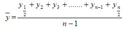
The average level in the interval series of dynamics ( ) is calculated by the simple arithmetic average formula:

• y - levels of the series ( y1, y2, ..., yn ),
• n is the number of periods (the number of levels of the series).

Consider the method of calculating the average level of the interval series of dynamics on the example of data on the sale of sugar in Russia.

Years	Sugar sold, thousand tons
1994	2905
1995	2585
1996	2647

- This is the average annual sales of sugar to the population of Russia for 1994-1996. In just three years, 8137 thousand tons of sugar was sold.

Torque Dynamics Series

The levels of momentary series of dynamics characterize the state of the phenomenon under study at certain points in time. Each subsequent level includes in whole or in part the previous figure. For example, the number of employees as of April 1, 1999 fully or partially includes the number of employees as of March 1.

If we add up these figures, we will get a repeated account of those workers who worked during the whole month. The resulting amount of the economic content does not have, this is a calculated indicator.

In the time series of dynamics with equal time intervals, the average level of the series is calculated by the average chronological formula:

• y - levels of the moment series;
• n is the number of moments (levels of the series);
• n - 1 - the number of time periods (years, quarters, months).

Consider the method of such calculation for the following data on the list of the number of employees for 1 quarter.

	Number of employees
on January 1	150
on February 1	145
on March 1	162
on April 1	166

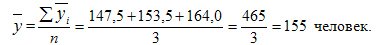
It is necessary to calculate the average level of a number of dynamics, in this example - the average list number of employees of the enterprise:

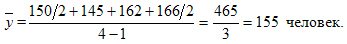
The calculation is made according to the average chronological formula. The average payroll number of employees for the 1st quarter was 155 people. In the denominator - 3 months in the quarter, and in the numerator (465) is an estimated number, it has no economic content. In the overwhelming number of economic calculations, months, regardless of the number of calendar days, are considered equal.

In the time series of dynamics with unequal time intervals, the average level of the series is calculated by the formula of the arithmetic average weighted. The length of time (t-days, months) is taken as the average weights. Perform a calculation using this formula.

The list number of employees of the enterprise for October is as follows: on October 1 - 200 people, on October 7, 15 people were received, 1 person was dismissed on October 12, 10 people were received on October 21 and there were no workers until the end of the month. This information can be represented as follows:

Number of employees	Number of days (time period)
200	6 (from 1 to 6 inclusive)
215	5 (from 7 to 11 inclusive)
214	9 (from 12 to 20 inclusive)
224	11 (from 21 to 31 inclusive)

When determining the average level of a series, it is necessary to take into account the duration of the periods between dates, i.e., apply the weighted arithmetic average formula:

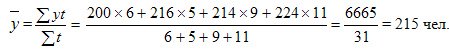
In this formula, the numerator ( ) has an economic content. In the above example, the numerator (6665 person-days) is the calendar fund of the enterprise’s employees in October. The denominator (31 days) is the calendar number of days in the month.

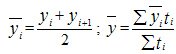
In those cases where we have a momentum series of dynamics with unequal time intervals, and the specific dates of the indicator change are unknown to the researcher, then we must first calculate the average value ( ) for each time interval using the simple average arithmetic formula, and then calculate the average level for the entire dynamics series, weighing the calculated average values ​​by the duration of the corresponding time interval . Formulas are as follows:

The time series considered above consist of absolute indicators obtained as a result of statistical observations. The originally constructed series of the dynamics of absolute indices can be transformed into series of derivatives: series of averages and series of relative values. The series of relative values ​​can be chain (as% of the previous period) and basic (as% of the initial period taken as the base of comparison - 100%). The calculation of the average level in the derived series of dynamics is performed using other formulas.

Medium range

First, we transform the moment dynamics series given above with equal time intervals into a series of average values. To do this, we calculate the average payroll number of employees for each month, as the average of the indicators at the beginning and end of the month ( ): January (150 + 145): 2 = 147.5; February (145 + 162): 2 = 153.5; March (162 + 166): 2 = 164.

Imagine this in tabular form.

Months	Average number of employees
January	147.5
February	153.5
March	164.0

The average level in the derived series of average values ​​is calculated by the formula of simple arithmetic:

It should be noted that the average payroll number of the company's employees for Q1, calculated using the average chronological formula based on the data on the 1st day of each month and the arithmetic average — according to the derived series — are equal to each other, i.e. 155 people. Comparison of calculations allows us to understand why in the formula of the average chronological, the initial and final levels of a series are taken at half the size, and all intermediate levels are taken at full size.

Series of averages, derived from moment or interval dynamics, should not be confused with series of dynamics, in which the levels are expressed as an average value. For example, the average yield of wheat by year, the average wage, etc.

Rows of relative values

In economic practice, very widely used series of relative values. Virtually any initial dynamic range can be converted to a series of relative values. In essence, transformation means the replacement of the absolute indicators of a series by the relative magnitudes of the dynamics.

The average level of a series in relative series of dynamics is called the average annual growth rate. Methods for its calculation and analysis are discussed below.

Analysis of time series

For a reasonable assessment of the development of phenomena in time, it is necessary to calculate the analytical indicators: absolute growth, growth rate, growth rate, growth rate, the absolute value of one percent increase.

The table shows a digital example, and below are formulas for the calculation and economic interpretation of indicators.

Analysis of the dynamics of the production of product "A" in the enterprise for 1994-1998.

Years	Produced KT	Absolute increments kt		Growth rates		The pace growth%		Growth rate,%		The value of 1% of growth, kt.
		Chain	basic	chains	basic	chains	basic	chains	basic
		3	four	five	6	7	eight	9	ten	eleven
1994	200	-	-	-	1.00	-	100	-	-	-
1995	210	ten	ten	1,050	1.05	105.0	105	5.0	5.0	2.00
1996	218	eight	18	1,038	1.09	103.8	109	3.8	9.0	2.10
1997	230	12	thirty	1,055	1.15	105.5	115	5.5	15.0	2.18
1998	234	four	34	1,017	1.17	101.7	117	1.7	17.0	2.30

Absolute increments ( Δy ) show how many units the subsequent level of the series has changed compared to the previous one (group 3. - chain absolute increments) or compared to the initial level (group 4. - basic absolute gains). Calculation formulas can be written as follows:

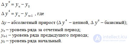
With a decrease in the absolute values ​​of the series will be, respectively, a "decrease", "decrease."

The absolute growth indices show that, for example, in 1998 the production of product “A” increased by 4 thousand tons compared to 1997, and by 34 thousand tons compared to 1994; for the remaining years, see table. 11.5 gr. 3 and 4.

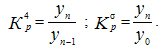
The growth rate shows how many times the level of the row has changed compared to the previous one (group 5 - chain growth or decline rates) or compared with the initial level (group 6 - base growth or decline rates). Calculation formulas can be written as follows:

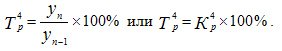
Growth rates show how much percent is the next level of the series compared to the previous one (group 7 - chain growth rates) or compared to the initial level (group 8 - basic growth rates). Calculation formulas can be written as follows:

So, for example, in 1997, the volume of production of the product "A" compared to 1996 amounted to 105.5% (

Growth rates show the percentage increase in the level of the reporting period compared with the previous one (gr.9 - chain growth rates) or compared with the initial level (gr.10 - basic growth rates). Calculation formulas can be written as follows:

Tpr = Tr - 100% or Tpr = absolute increase / level of the previous period * 100%

So, for example, in 1996 compared to 1995, product "A" produced more by 3.8% (103.8% - 100%) or (8: 210) x100%, and compared to 1994 - by 9% (109% - 100%).

If the absolute levels in the series decrease, the rate will be less than 100% and, accordingly, there will be a decrease rate (growth rate with a minus sign).

The absolute value of a 1% increase (c. 11) shows how many units need to be produced in a given period so that the level of the previous period increased by 1%. In our example, in 1995 it was necessary to produce 2.0 thousand tons, and in 1998 - 2.3 thousand tons, i.e. much bigger.

To determine the magnitude of the absolute value of 1% growth in two ways:

• the level of the previous period divided by 100;
• chain absolute increments divided by the corresponding chain rates of growth.

Absolute value of 1% increase =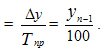

In the dynamics, especially over a long period, a joint analysis of the growth rates with the content of each percent increase or decrease is important.

Note that the considered methodology for analyzing the dynamics series is applicable both for dynamics series whose levels are expressed in absolute values ​​(t, thousand rubles, number of employees, etc.) and for dynamics series whose levels are expressed in relative indicators (% of marriage ,% of the ash content of coal, etc.) or average values ​​(average yield in kg / ha, average wages, etc.).

Along with the considered analytical indicators, calculated for each year in comparison with the previous or initial level, when analyzing the time series, it is necessary to calculate the average for the period analytical indicators: the average level of the series, the average annual absolute increase (decrease) and the average annual growth rate and growth rate.

Methods for calculating the average level of a number of dynamics were discussed above. In the interval range of dynamics under consideration, the average level of a series is calculated by the formula of the simple arithmetic mean:

The average annual production of the product for 1994-1998. amounted to 218.4 thousand tons

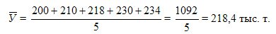
The average annual absolute growth is also calculated by the simple arithmetic average formula:

Annual absolute increments varied over the years from 4 to 12 thousand tons (see gr. 3), and the average annual increase in production for the period 1995-1998. amounted to 8.5 thousand tons

Methods for calculating the average growth rate and average growth rate require more detailed consideration. Consider them on the example given in the table of annual indicators of row level.

Average annual growth rate and average annual growth rate

First of all, we note that the growth rates given in the table (groups 7 and 8) are series of relative values ​​of the dynamics — derivatives of the interval series of dynamics (group 2). Annual growth rates (c.7) vary by year (105%; 103.8%; 105.5%; 101.7%). How to calculate the average of annual growth rates? This value is called the average annual growth rate.

The average annual growth rate is calculated in the following sequence:

1. First, the average annual growth rate (decline) is calculated using the geometric average formula:
2. on the basis of the average annual rate, the average annual growth rate is determined ( ) by multiplying the coefficient by 100%:

Average annual growth rate ( determined by subtracting from the growth rate of 100%.

The average annual growth rate (reduction) according to the geometric average formula can be calculated in two ways:

1) on the basis of the absolute indicators of a number of dynamics according to the formula:

• n is the number of levels;
• n - 1 - the number of years in the period;

2) on the basis of annual growth factors according to the formula

• m is the number of coefficients.

The results of calculation by the formulas are equal, since in both formulas the exponent is the number of years in the period during which the change occurred. And the radical expression is the rate of growth of the indicator for the entire period of time (see table. 11.5, c.6, on the line for 1998).

The average annual growth rate is

The average annual growth rate is determined by subtracting 100% from the average annual growth rate. В нашем примере среднегодовой темп прироста равен

Следовательно, за период 1995 — 1998 гг. объем производства продукта "А" в среднем за год возрастал на 4,0%. Ежегодные темпы прироста колебались от 1,7% в 1998 г. до 5,5% в 1997 г. (за каждый год темпы прироста см. в табл. 11.5, гр. 9).

Среднегодовой темп роста (прироста) позволяет сравнивать динамику развития взаимосвязанных явлений за длительный период времени (например, среднегодовые темпы роста численности работающих по отраслям экономики, объема производства продукции и др.), сравнивать динамику какого-либо явления по разным странам, исследовать динамику какого-либо явления по периодам исторического развития страны.

Анализ сезонных колебаний

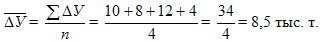
Изучение сезонных колебаний проводится с целью выявления закономерно повторяющихся различий в уровне рядов динамики в зависимости от времени года. Так, например, реализация сахара населению в летний период значительно возрастает в связи с консервированием фруктов и ягод. Потребность в рабочей силе в сельскохозяйственном производстве различна в зависимости от времени года. Задача статистики состоит в том, чтобы измерить сезонные различия в уровне показателей, а чтобы выявленные сезонные различия были закономерными (а не случайными) необходимо строить анализ на базе данных за несколько лет, по крайней мере не менее чем за три года. In tab. 11.6 приведены исходные данные и методика анализа сезонных колебаний методом простой средней арифметической.

Средняя величина за каждый месяц исчисляется по формуле средней арифметической простой. Например, за январь 2202 = (2106 +2252 +2249):3.

Индекс сезонности ( табл. 11.5 гр.7.) исчисляется путем деления средних величин за каждый месяц на общую среднюю месячную величину, принятую за 100%. Средняя месячная за весь период может быть исчислена путем деления общего расхода горючего за три года на 36 месяцев (1188082 т : 36 = 3280 т) или путем деления на 12 суммы средних месячных, т.е. суммарного итога по гр. 6 (2022 + 2157 + 2464 и т.д. + 2870) : 12.

Таблица 11.6 Сезонные колебания потребления горючего в сельскохозяйственных предприятиях района за 3 года

Месяцы	Расход горючего, тонн			Сумма за 3 года, т (2+3+4)	Средняя месячная за 3 года, т	Индекс сезонности, %
	1 year	2 год	3 год
one	2	3	four	five	6	7
January	2106	2252	2249	6607	2202	67,1
February	2120	2208	2142	6470	2157	65.7
March	2300	2580	2512	7392	2464	75,1
April	3056	3300	3412	9768	3256	99,2
May	3380	3440	3469	10289	3430	104.6
June	4044	4210	4210	12464	4155	126,6
July	4280	4184	4296	12760	4253	130,0
August	4088	4046	4020	12154	4051	123,5
September	3604	3622	3631	10857	3619	110,3
October	3818	3636	3583	11037	3679	112,1
November	3120	3218	3336	9674	3224	98,3
December	2778	2802	3030	8610	2870	87,5
Total	38694	39498	39890	118082	3280	100.0

Fig. 11.1. Сезонные колебания потребления горючего в сельскохозяйственных предприятиях за 3 года.

Для наглядности на основе индексов сезонности строится график сезонной волны (рис. 11.1). По оси абсцисс располагают месяцы, а по оси ординат — индексы сезонности в процентах (табл. 11.6, гр.7). Общая средняя месячная за все годы располагается на уровне 100%, а средние месячные индексы сезонности в виде точек наносят на поле графика в соответствии с принятым масштабом по оси ординат.

Точки соединяют между собой плавной ломаной линией.

В приведенном примере годовые объемы расхода горючего различаются незначительно. Если же в ряду динамики наряду с сезонными колебаниями имеется ярко выраженная тенденция роста (снижения), т.е. уровни в каждом последующем году систематически значительно возрастают (уменьшаются) по сравнению с уровнями предыдущего года, то более достоверные данные о размерах сезонности получим следующим образом:

1. для каждого года вычислим среднюю месячную величину;
2. исчислим индексы сезонности за каждый год путем деления данных за каждый месяц на среднюю месячную величину за этот год и умножения на 100%;
3. за весь период исчислим средние индексы сезонности по формуле средней арифметической простой из исчисленных за каждый год месячных индексов сезонности. Так, например, за январь средний индекс сезонности получим, если сложим январские значения индексов сезонности за все годы (допустим за три года) и разделим на число лет, т.е. на три. Аналогично исчислим за каждый месяц средние индексы сезонности.

Переход за каждый год от абсолютных месячных значений показателей к индексам сезонности позволяет устранить тенденцию роста (снижения) в ряду динамики и более точно измерить сезонные колебания.

В условиях рынка при заключении договоров на поставку различной продукции (сырья, материалов, электроэнергии, товаров) необходимо располагать информацией о сезонных потребностях в средствах производства, о спросе населения на отдельные виды товаров. Результаты исследования сезонных колебаний важны для эффективного управления экономическими процессами.

Приведение рядов динамики к одинаковому основанию

В экономической практике часто возникает необходимость сравнения между собой нескольких рядов динамики (например, показатели динамики производства электроэнергии, производства зерна, продажи легковых автомобилей и др.). Для этого нужно преобразовать абсолютные показатели сравниваемых рядов динамики в производные ряды относительных базисных величин, приняв показатели какого-либо одного года за единицу или за 100%.Такое преобразование нескольких рядов динамики называется приведением их к одинаковому основанию. Теоретически за базу сравнения может быть принят абсолютный уровень любого года, но в экономических исследованиях для базы сравнения надо выбирать период, имеющий определенное экономическое или историческое значение в развитии явлений. В настоящее время за базу сравнения целесообразно принять, например, уровень 1990 г.

Alignment Dynamics Series Methods

Для исследования закономерности (тенденции) развития изучаемого явления необходимы данные за длительный период времени. Тенденцию развития конкретного явления определяет основной фактор. Но наряду с действием основного фактора в экономике на развитие явления оказывают прямое или косвенное влияние множество других факторов, случайных, разовых или периодически повторяющихся (годы, благоприятные для сельского хозяйства, засушливые и т.п.). Практически все ряды динамики экономических показателей на графике имеют форму кривой, ломаной линии с подъемами и снижениями. Во многих случаях по фактическим данным ряда динамики и по графику трудно определить даже общую тенденцию развития. Но статистика должна не только определить общую тенденцию развития явления (рост или снижение), но и дать количественные (цифровые) характеристики развития.

The tendencies of the development of phenomena are studied by the methods of leveling the dynamic series:

• Interval Enlargement Method
• Moving average method
• Analytical alignment method

In tab.11.7 (Group 2) shows actual data on grain production in Russia for 1981-1992. (in all categories of farms, in weight after refinement) and calculations to level this series by three methods.

The method of integration of time intervals (gr. 3).

Учитывая, что ряд динамики небольшой, интервалы взяты трехлетние и для каждого интервала исчислены средние. Среднегодовой объем производства зерна по трехлетним периодам исчислен по формуле средней арифметической простой и отнесен к среднему году соответствующего периода. Так, например, за первые три года (1981 — 1983 гг.) средняя записана против 1982 г.: (73,8+ 98,0+104,3) : 3= 92,0 (млн. т). За следующий трехлетний период (1984 — 1986 гг.) средняя (85,1 +98,6+ 107,5) : 3= 97,1 млн. т записана против 1985 г.

За остальные периоды результаты расчета в гр. 3

Приведенные в гр. 3 показатели среднегодового объема производства зерна в России свидетельствуют о закономерном увеличении производства зерна в России за период 1981 — 1992 гг.

Метод скользящей средней

Метод скользящей средней (см. гр. 4 и 5) также основан на исчислении средних величин за укрупненные периоды времени. Цель та же — абстрагироваться от влияния случайных факторов, взаимопогасить их влияние в отдельные годы. Но метод расчета другой.

В приведенном примере исчислены пятизвенные (по пятилетним периодам) скользящие средние и отнесены к серединному году в соответствующем пятилетнем периоде. Так, за первые пять лет (1981-1985 гг.) по формуле средней арифметической простой исчислен среднегодовой объем производства зерна и записан в табл. 11.7 против 1983 г.(73,8+ 98,0+ 104,3+ 85,1+ 98,6): 5= 92,0 млн. т; за второй пятилетний период (1982 — 1986 гг.) результат записан против 1984 г. (98,0 + 104,3 +85,1 + 98,6 + 107,5):5 =493,5:5 = 98,7 млн. т.

За последующие пятилетние периоды расчет производится аналогичным способом путем исключения начального года и прибавления следующего за пятилетним периодом года и деления полученной суммы на пять. При этом методе концы ряда остаются пустыми.

Какой продолжительности должны быть периоды времени? Три, пять, десять лет? Вопрос решает исследователь. В принципе, чем больше период, тем больше происходит сглаживание. Но надо учитывать длину ряда динамики; не забывать, что метод скользящей средней оставляет срезанные концы выравненного ряда; учитывать этапы развития, например, в нашей стране долгие годы социально-экономическое развитие планировалось и соответственно анализировалось по пятилеткам.

Таблица 11.7 Выравнивание данных о производстве зерна в России за 1981 — 1992 гг.

Годы	Произведено, млн. т	Средняя за 3 года, млн. т	Скользящая сумма за 5 лет, млн. т		Расчетные показатели
			Amount	Average
one	2	3	four	five	6	7	eight	9
1981	73.8	-	-	-	one	one	73,8	89.5
1982	98,0	92,0	-	-	2	four	196,0	91,1
1983	104,3	-	459,8	92,0	3	9	312,9	92,6
1984	85,1	-	493,5	98,7	four	sixteen	340,4	94.2
1985	98.6	97,1	494.1	98,8	five	25	493,0	95,8
1986	107.5	-	483.5	96,7	6	36	645,0	97,3
1987	98.6	-	503,2	100,6	7	49	690,2	98.9
1988	93,7	99,1	521,3	104,3	eight	64	749.6	100,4
1989	104,8	-	502,9	100,6	9	81	943,2	102,0
1990	116,7	-	511,2	102.2	ten	100	1167,0	103.5
1991	89,1	104,2	-	-	eleven	121	980,1	105,1
1992	106.9	-	-	-	12	144	1282,8	106,7
Total	1177,1	-	-	-	78	650	7874,0	1177,1

Метод аналитического выравнивания

Метод аналитического выравнивания (гр.6 — 9) основан на вычислении значений выравненного ряда по соответствующим математическим формулам. In tab. 11.7 приведены вычисления по уравнению прямой линии:

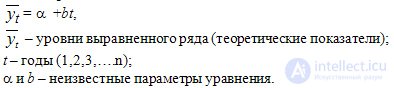
Для определения параметров надо решить систему уравнений:

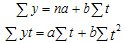
Необходимые величины для решения системы уравнений вычислены и приведены в таблице (см. гр.6 — 8), подставим их в уравнение:

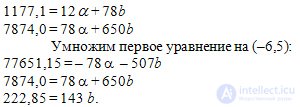
В результате вычислений получаем: α= 87,96; b = 1,555 .

Подставим значение параметров и получим уравнение прямой:

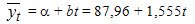
Для каждого года подставляем значение t и получаем уровни выравненного ряда (см. гр.9):

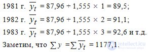
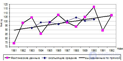
Fig. 11.2. Производство зерна в России за 1981-1982 гг.

В выравненном ряду происходит равномерное возрастание уровней ряда в среднем за год на 1,555 млн.т (значение параметра "b"). Метод основан на абстрагировании влияния всех остальных факторов, кроме основного.

Phenomena can develop in dynamics evenly (increase or decrease). In these cases, the straight line equation is most often suitable. If development is uneven, for example, at first a very slow growth, and from a certain moment a sharp increase, or, conversely, a sharp decrease, and then a slowdown in the decline, then the alignment must be performed using other formulas (parabola, hyperbola, etc.). If necessary, refer to textbooks on statistics or special monographs, where the choice of a formula to adequately reflect the actual trend of the studied dynamics is set out in greater detail.

For clarity, the indicators of the levels of the actual series of dynamics and aligned rows are plotted on the graph (Fig. 11.2). The actual data is a broken line in black, indicating a rise and decrease in the volume of grain production. The remaining lines on the graph show that the use of the moving average method (line with cut ends) allows to significantly align the levels of the dynamic series and, accordingly, make the broken curve line smoother and smoother on the graph. However, the aligned lines still remain curved lines. Constructed on the basis of the theoretical values ​​of a series obtained by mathematical formulas, the line strictly corresponds to a straight line.

Each of the three considered methods has its advantages, but in most cases the method of analytical alignment is preferable. However, its use is associated with large computational work: solving a system of equations; checking the validity of the selected function (form of communication); calculation of the levels of the aligned series; the construction of the schedule. For the successful implementation of such work, it is advisable to use a computer and appropriate programs.