7.5. Alignment of statistical series

In any statistical distribution, inevitably there are elements of randomness, due to the fact that the number of observations is limited, that it was those, and not other experiments that gave precisely those, and not other results. Only with a very large number of observations, these elements of randomness are smoothed out, and the random phenomenon reveals a fully inherent pattern. In practice, we almost never deal with such a large number of observations and are forced to reckon with the fact that any statistical distribution is characterized by more or less random features. Therefore, when processing statistical material, it is often necessary to decide how to select a theoretical distribution curve for a given statistical series, expressing only the essential features of statistical material, but not randomness, associated with an insufficient amount of experimental data. Such a task is called the task of leveling (smoothing) the statistical series.

The task of alignment is to find a theoretical smooth distribution curve that, from one point of view, best describes this statistical distribution (Fig. 7.5.1).

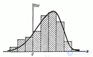
Fig. 7.5.1

The problem of the best alignment of statistical series, as well as the problem of the best analytical representation of empirical functions in general, is a task that is largely uncertain, and its solution depends on what is agreed to be considered “best”. For example, when smoothing empirical dependencies, very often they proceed from the so-called principle or the method of least squares (see 14.5), considering that the best approximation to the empirical dependence in this class of functions is one in which the sum of the squares of the deviations turns to a minimum. In this case, the question of which class of functions the best approximation should be sought for is decided not from mathematical considerations, but from considerations related to the physics of the problem being solved, taking into account the nature of the empirical curve obtained and the degree of accuracy of the observations made. Often, the fundamental nature of the function expressing the dependence under investigation is known in advance from theoretical considerations, but from experience only some numerical parameters are required to be included in the function expression; These parameters are selected using the method of least squares.

The situation is similar with the task of leveling statistical series. As a rule, the fundamental form of a theoretical curve is chosen in advance from considerations related to the essence of the problem, and in some cases simply with the appearance of the statistical distribution. The analytical expression of the selected distribution curve depends on some parameters; the task of leveling the statistical series goes into the problem of rational choice of those values ​​of the parameters for which the correspondence between the statistical and theoretical distributions turns out to be the best.

Suppose, for example, that the quantity studied there is a measurement error resulting from the summation of the effects of a set of independent elementary errors; then from theoretical considerations we can assume that the value obeys the normal law:

(7.5.1)

and the alignment problem goes into the problem of the rational choice of parameters and in expression (7.5.1).

There are cases when it is known in advance that it is distributed statistically approximately evenly over a certain interval; then you can pose the problem of a rational choice of the parameters of the law of uniform density

which can best replace (equalize) the specified statistical distribution.

It should be borne in mind that any analytical function , with the help of which the statistical distribution is aligned, should have the main properties of the density distribution:

(7.5.2)

Suppose that, based on certain considerations, we have chosen the function satisfying conditions (7.5.2), with the help of the bark we want to equalize this statistical distribution; The expression of this function includes several parameters. ; It is required to select these parameters so that the function best described this statistical material. One of the methods used to solve this problem is the so-called method of moments.

According to the method of moments, the parameters are chosen in such a way that several of the most important numerical characteristics (moments) of the theoretical distribution are equal to the corresponding statistical characteristics. For example, if the theoretical curve depends only on two parameters and , these parameters are chosen so that the expectation and variance theoretical distribution coincided with the corresponding statistical characteristics and . If the curve depends on three parameters, you can choose them so that the first three points coincide, etc. When aligning statistical series, a specially developed system of Pearson curves, each of which depends in general on four parameters, may be useful. When aligning, these parameters are selected so as to preserve the first four points of the statistical distribution (expectation, variance, third and fourth moments). The original set of distribution curves constructed by a different principle was given by N.A. Borodachev. The principle on which the N.A. Borodachev, lies in the fact that the choice of the type of theoretical curve is not based on external formal features, but on an analysis of the physical essence of a random phenomenon or process leading to a particular distribution law.

It should be noted that when aligning the statistical series, it is not rational to use moments of order higher than four, since the accuracy of the calculation of the moments drops sharply with increasing order.

Example. 1. In 7.3 shows the statistical distribution of lateral interference errors when shooting from an airplane at a ground target. It is required to level this distribution using normal law:

.

Normal law depends on two parameters: and . We select these parameters so as to preserve the first two points — the expectation and variance — of the statistical distribution.

Let us calculate the approximate statistical average of the error of the pickup using the formula (7.47), and for the representative of each digit we take its middle:

To determine the variance, we first calculate the second initial moment using the formula (7.4.9), assuming

Using the expression of dispersion through the second initial moment (formula (7.4.6)), we get:

Choose parameters and normal law so that the conditions are met:

that is, take:

.

Write the expression of the normal law:

Using the table. 3 applications, calculate the values on the borders of discharges

Let us construct a histogram on one graph (fig. 7.5.2) and a distribution curve leveling it.

The graph shows that the theoretical distribution curve while preserving, in general, the essential features of the statistical distribution, it is free from random irregularities in the course of the histogram, which, apparently, can be attributed to random reasons; a more serious justification of the last judgment will be given in the next paragraph.

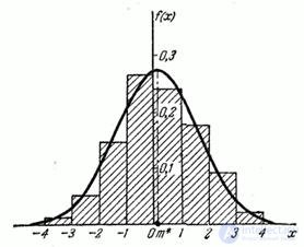
Fig. 7.5.2

Note. In this example, when determining , we used the expression (7.4.6) of statistical variance through the second initial moment. This technique can be recommended only in the case when the expectation investigated random variable relatively small; otherwise, the formula (7.4.6) expresses the variance as a difference of close numbers and gives a very low accuracy. In the case that this is the case, it is recommended to either calculate directly by the formula (7.4.3), or move the origin to some point close to and then apply the formula (7.4.6). Using formula (7.4.3) is equivalent to transferring the origin to a point ; this can be inconvenient because the expression can be fractional and subtraction of each while unnecessarily complicates the calculations; therefore it is recommended to transfer the origin to some round value close to .

Example 2. In order to investigate the law of the distribution of the error in measuring the distance using a radio-range meter, 400 distance measurements were made. The results of the experiments are presented in the form of a statistical series:

Align the statistical series using the law of uniform density.

Decision. The law of uniform density is expressed by the formula

and depends on two parameters and . These parameters should be chosen so as to preserve the first two points of the statistical distribution - the expectation and variance . From example 5.8 we have the expression of the expectation and variance for the law of uniform density:

In order to simplify the calculations associated with the determination of statistical moments, we move the origin to the point and take for the representative of his rank his middle. The distribution series is:

Where - the average for the discharge value of the radio range meter with a new origin.

Approximate value of statistical average error equally:

Second statistical moment of magnitude equals:

,

whence statistical variance:

.

Turning to the previous reference point, we get a new statistical average:

in the same statistical variance:

.

The parameters of the law of uniform density are determined by the equations:

.

Solving these equations for and , we have:

,

from where

.

In fig. 7.5.3. shows the histogram and the law of uniform density equalizing it .

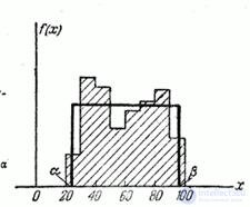
Fig. 7.5.3