Lecture
The method of least squares (OLS, Eng. Ordinary Least Squares, OLS ) is a mathematical method used to solve various problems, based on minimizing the sum of squares of deviations of some functions from the desired variables. It can be used to "solve" overdetermined systems of equations (when the number of equations exceeds the number of unknowns), to search for solutions in the case of ordinary (not overdetermined) nonlinear systems of equations, to approximate point values with a function. OLS is one of the basic regression analysis methods for estimating unknown parameters of regression models from sample data.
Until the beginning of the XIX century. Scientists did not have certain rules for solving a system of equations in which the number of unknowns is less than the number of equations; until that time, private methods were used, depending on the type of equations and the wit of the calculators, and therefore different calculators, based on the same observational data, came to different conclusions. Gauss (1795) owned the first application of the method, and Legendre (1805) independently discovered and published it under the modern name (fr. Méthode des moindres quarrés ) [1] . Laplace connected the method with the theory of probability, and the American mathematician Edrein (1808) considered his probability-theoretic applications [2] . The method is distributed and improved by further research Enke, Bessel, Ganzen and others.
The work of A. A. Markov at the beginning of the 20th century allowed the least squares method to be included in the theory of estimation of mathematical statistics, in which it is an important and natural part. Through the efforts of J. Neumann, F. David, A. Aitken, S. Rao, many important results were obtained in this area [3] .
Let be  - set
- set  unknown variables (parameters),
  - a set of functions from this set of variables. The task is to select such values of x so that the values of these functions are as close as possible to some values.
  . Essentially we are talking about the "solution" of the overdetermined system of equations
  in the indicated sense of maximum proximity of the left and right parts of the system. The essence of MNCs is to choose as the "measure of proximity" the sum of squared deviations of the left and right sides -
  . Thus, the essence of MNCs can be expressed as follows:

If the system of equations has a solution, then the minimum of the sum of squares will be zero and exact solutions of the system of equations can be found analytically or, for example, by various numerical optimization methods. If the system is redefined, that is, speaking loosely, the number of independent equations is greater than the number of variables sought, then the system does not have an exact solution and the least squares method allows us to find some "optimal" vector in the sense of maximum proximity of vectors  and
and  or maximum proximity of the vector of deviations
  to zero (proximity is understood in the sense of the Euclidean distance).
In particular, the method of least squares can be used to "solve" a system of linear equations
 ,
,
where is the matrix  not square, but rectangular in size
  (more precisely, the rank of the matrix A is greater than the number of sought variables).
Such a system of equations, in general, has no solution. Therefore, this system can be “solved” only in the sense of choosing such a vector to minimize the "distance" between vectors  and
and  . To do this, you can apply the criterion for minimizing the sum of squares of the differences of the left and right sides of the equations of the system, that is,
  . It is easy to show that the solution of this minimization problem leads to the solution of the following system of equations

Using the pseudoinverse operator, the solution can be rewritten as:
 ,
,
Where  - pseudo-inverse matrix for .
This problem can also be “solved” using the so-called weighted OLS (see below), when different equations of the system get different weights from theoretical considerations.
Strict justification and determination of the limits of the substantive applicability of the method are given by A. A. Markov and A. N. Kolmogorov.
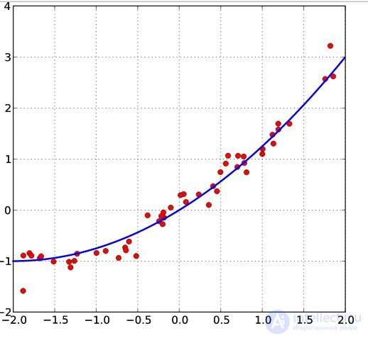
Let there be  values of some variable (these may be the results of observations, experiments, etc.) and the corresponding variables . The challenge is to interconnect between and approximate by some function
  known up to some unknown parameters i.e. actually find the best parameter values maximally approximating values to actual values . In fact, it comes down to the case of the “solution” of the redefined system of equations for :
In regression analysis, and in particular in econometrics, probabilistic models of dependencies between variables are used.
Where  - the so-called random model errors .
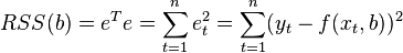
Accordingly, the deviations of the observed values from model already assumed in the model itself. The essence of the MNC (ordinary, classical) is to find such parameters for which the sum of squared deviations (errors, for regression models, they are often called regression residues)  will be minimal:

Where  - English Residual Sum of Squares [4] is defined as:
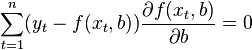
In the general case, this problem can be solved by numerical optimization (minimization) methods. In this case, they speak of non-linear OLS (NLS or NLLS - Non-Linear Least Squares ). In many cases, you can get an analytical solution. To solve the minimization problem, it is necessary to find the stationary points of the function  by differentiating it by unknown parameters , equating the derivatives to zero and solving the resulting system of equations:
Let the regression dependence be linear:

Let y be the observational column vector of the explained variable, and  - this
  - Matrix of observations of factors (matrix rows - vectors of values of factors in a given observation, column by column - a vector of values of this factor in all observations). The matrix representation of the linear model is:

Then the vector of estimates of the variable being explained and the vector of the regression residuals will be equal

accordingly, the sum of squares of the regression residuals will be equal to

Differentiating this function by parameter vector and equating the derivatives to zero, we obtain the system of equations (in matrix form):
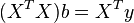 .
.
In the decoded matrix form, this system of equations is as follows:
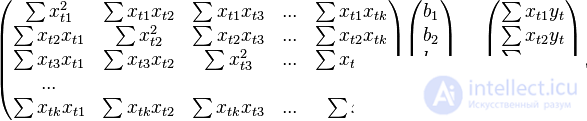 where all sums are taken for all valid values
  .
.
If a constant is included in the model (as usual), then  for all therefore, the number of observations is in the upper left corner of the matrix of the system of equations , and in the remaining elements of the first row and first column - just the sum of the values of the variables:
  and the first element of the right side of the system -
  .
.
The solution of this system of equations gives the general formula of least-squares estimate for a linear model:

For analytical purposes, the last representation of this formula turns out to be useful (in the system of equations when dividing by n, arithmetic averages appear instead of sums). If in the regression model the data is centered , then in this view the first matrix has the meaning of a selective covariance matrix of factors, and the second is the vector of covariances of factors with the dependent variable. If, in addition, the data are also normalized to the MSE (that is, ultimately standardized ), then the first matrix has the meaning of a selective correlation matrix of factors, the second vector is the vector of selective correlations of factors with a dependent variable.
An important property of the least-squares estimate for models with a constant is that the constructed regression line passes through the center of gravity of the sample data, that is, the equality is fulfilled:

In particular, in the extreme case, when the only regressor is a constant, we find that the least-squares estimate of a single parameter (the constant itself) is equal to the average value of the variable explained. That is, the arithmetic average, known for its good properties from the laws of large numbers, is also an OLS-estimate — it satisfies the criterion of the minimum of the sum of squares of deviations from it.
In the case of pairwise linear regression  when the linear dependence of one variable on another is evaluated, the calculation formulas are simplified (you can do without matrix algebra). The system of equations is:
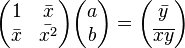
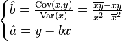
From here it is easy to find estimates of the coefficients:
Despite the fact that, in the general case, models with a constant are preferable, in some cases it is known from theoretical considerations that the constant  must be zero. For example, in physics, the relationship between voltage and amperage is
  ; Measuring voltage and amperage, it is necessary to evaluate the resistance. In this case, it is a model
  . In this case, instead of a system of equations, we have a single equation
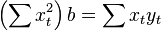
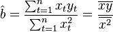
Therefore, the formula for estimating a single coefficient is
First of all, we note that for linear models, OLS-estimates are linear estimates, as follows from the above formula. For the inconsistency of the OLS estimates, it is necessary and sufficient to fulfill the most important condition of the regression analysis: the conditional on the factors of the mathematical expectation of a random error should be zero. This condition, in particular, is satisfied if
The first condition can always be considered fulfilled for models with a constant, since the constant assumes a nonzero expectation of errors (therefore, models with a constant are preferable in general).
The second condition - the condition of exogenous factors - is fundamental. If this property is not fulfilled, then we can assume that practically any estimates will be extremely unsatisfactory: they will not even be consistent (that is, even a very large amount of data does not allow obtaining qualitative assessments in this case). In the classical case, a stronger assumption is made about the determinism of factors, in contrast to a random error, which automatically means that the exogeneity condition is satisfied. In the general case, for the consistency of the estimates, it suffices to fulfill the exogeneity condition along with the convergence of the matrix  to some non-degenerate matrix with increasing sample size to infinity.
In addition to consistency and unbiasedness, the (ordinary) OLS estimates are also effective (the best in the class of linear unbiased estimates) it is necessary to perform additional properties of random error:

These assumptions can be formulated for the covariance matrix of the random error vector 
A linear model satisfying such conditions is called a classical one . OLS estimates for classical linear regression are unbiased, consistent and most effective estimates in the class of all linear unbiased estimates (in the English-language literature the abbreviation BLUE ( Best Linear Unbiased Estimator ) is sometimes used) —The Gaussian-Markov theorem ). As it is easy to show, the covariance matrix of the coefficient estimates vector will be equal to:
Efficiency means that this covariance matrix is “minimal” (any linear combination of coefficients, and in particular the coefficients themselves, have minimal variance), that is, in the class of linear unbiased estimates, the least-squares estimate is the best. The diagonal elements of this matrix — the variances of the coefficient estimates — are important parameters for the quality of the estimates obtained. However, it is impossible to calculate the covariance matrix, since the variance of random errors is unknown. It can be proved that the unbiased and consistent (for the classical linear model) estimate of the variance of random errors is:

Substituting this value into the formula for the covariance matrix and obtain an estimate of the covariance matrix. The estimates obtained are also unbiased and consistent. It is also important that the estimation of the error variance (and hence the coefficient dispersions) and the estimates of the model parameters are independent random variables, which makes it possible to obtain test statistics for testing hypotheses about the model coefficients.
It should be noted that if the classical assumptions are not fulfilled, the least-squares parameter estimates are not the most effective estimates (remaining unbiased and consistent). However, the assessment of the covariance matrix worsens even more - it becomes biased and untenable. This means that the statistical conclusions about the quality of the constructed model in this case may be extremely unreliable. One of the solutions to the latter problem is the use of special estimates of the covariance matrix, which are consistent with violations of the classical assumptions (standard errors in the form of White and standard errors in the form of Newey-West). Another approach is to use the so-called generalized OLS.
The least squares method allows for a broad generalization. Instead of minimizing the sum of squares of residuals, you can minimize some positive-definite quadratic form of the residual vector where
where  - some symmetric positive definite weight matrix. The usual OLS is a special case of this approach, when the weight matrix is proportional to the identity matrix. As is known from the theory of symmetric matrices (or operators) for such matrices there is a decomposition
 .Therefore, this functional can be represented as follows
  , that is, this functional can be represented as the sum of the squares of some transformed "residues". Thus, we can distinguish a class of least squares methods - LS-methods (Least Squares).
It has been proved (Aitken's theorem) that for the generalized linear regression model (in which no restrictions are imposed on the covariance matrix of random errors) the most effective (in the class of linear unbiased estimates) are the estimates of the so-called. Generalized OLS (OMNK, GLS - Generalized Least Squares) - LS method with a weight matrix equal to the inverse random error covariance matrix: .
.
It can be shown that the formula of the OMNK estimates of the parameters of the linear model is

Ковариационная матрица этих оценок соответственно будет равна

Фактически сущность ОМНК заключается в определенном (линейном) преобразовании (P) исходных данных и применении обычного МНК к преобразованным данным. Цель этого преобразования — для преобразованных данных случайные ошибки уже удовлетворяют классическим предположениям.
В случае диагональной весовой матрицы (а значит и ковариационной матрицы случайных ошибок) имеем так называемый взвешенный МНК (WLS — Weighted Least Squares). В данном случае минимизируется взвешенная сумма квадратов остатков модели, то есть каждое наблюдение получает «вес», обратно пропорциональный дисперсии случайной ошибки в данном наблюдении: 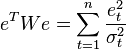 . Фактически данные преобразуются взвешиванием наблюдений (делением на величину, пропорциональную предполагаемому стандартному отклонению случайных ошибок), а к взвешенным данным применяется обычный МНК.

Comments
To leave a comment
Probability theory. Mathematical Statistics and Stochastic Analysis
Terms: Probability theory. Mathematical Statistics and Stochastic Analysis