17.2. Spectral decomposition of a stationary random function on a finite time interval. Dispersion spectrum

On the two examples given in the previous we clearly saw that there is a connection between the nature of the correlation function and the internal structure of the corresponding random process. Depending on which frequencies and in which ratios prevail in the composition of a random function, its correlation function has one or the other. From such considerations, we directly come to the concept of the spectral composition of a random function.

The concept of "spectrum" is found not only in the theory of random functions; It is widely used in mathematics, physics and engineering.

If any oscillatory process is represented as a sum of harmonic oscillations of various frequencies (the so-called “harmonics”), then the spectrum of the oscillatory process is a function describing the amplitude distribution over different frequencies. The spectrum shows what kind of fluctuations prevail in this process, what is its internal structure.

A completely analogous spectral description can also be given to a stationary random process; the difference is that for a random process, the amplitudes of the oscillations will be random variables. The spectrum of the stationary random function will describe the dispersion distribution at different frequencies.

Let us approach the concept of the spectrum of a stationary random function from the following considerations.

Consider the stationary random function which we observe on the interval (fig. 17.2.1).

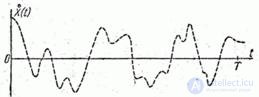
Fig. 17.2.1.

The correlation function of the random function is given.

.

Function There is an even function:

and, therefore, a symmetric curve is displayed on the graph (fig. 17.2.2).

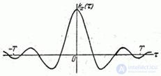
Fig. 17.2.2.

When it changes and from before argument varies from before .

We know that the even function on the interval can be decomposed into a Fourier series using only even (cosine) harmonics:

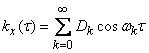, (17.2.1)

Where

; , (17.2.2)

and coefficients are determined by the formulas:

(17.2.3)

Bearing in mind that the functions and even, you can convert formulas (17.2.3) to the form:

(17.2.4)

We turn in the expression (17.2.1) of the correlation function from argument again to two arguments and . For this we set

(17.2.5)

and substitute the expression (17.2.5) into the formula (17.2.1):

. (17.2.6)

We see that expression (17.2.6) is nothing more than a canonical decomposition of the correlation function . The coordinate functions of this canonical expansion are alternately the cosines and sines of frequencies that are multiples of :

.

We know that from the canonical decomposition of the correlation function, we can construct a canonical decomposition of the random function itself with the same coordinate functions and with dispersions equal to the coefficients in the canonical decomposition of the correlation function.

Therefore, the random function can be represented as canonical decomposition:

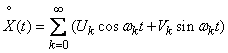, (17.2.7)

Where - uncorrelated random variables with a mathematical expectation equal to zero and variances that are the same for each pair of random variables with the same index :

. (17.2.8)

Dispersions at various are determined by formulas (17.2.4).

So we got on the interval canonical decomposition of a random function whose coordinate functions are functions , at various . A decomposition of this kind is called the spectral decomposition of a stationary random function. The so-called spectral theory of stationary random processes is based on the representation of random functions in the form of spectral expansions.

The spectral decomposition depicts a stationary random function decomposed into harmonic oscillations of various frequencies:

moreover, the amplitudes of these oscillations are random variables.

Determine the variance of the random function given by spectral decomposition (17.2.7). By the theorem on the dispersion of a linear function of uncorrelated random variables

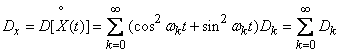. (17.2.9)

Thus, the variance of a stationary random function is equal to the sum of the variances of all the harmonics of its spectral decomposition. Formula (17.2.9) shows that the variance of the function In a known manner, it is distributed over different frequencies: one dispersion corresponds to larger dispersions, to the other - smaller ones. The distribution of dispersions over frequencies can be illustrated graphically in the form of the so-called spectrum of a stationary random function (more precisely, the spectrum of dispersions). For this purpose, the frequencies are plotted on the abscissa axis. , and on the ordinate axis - the corresponding dispersion (Fig. 17.2.3).

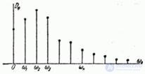
Fig. 17.2.3.

Obviously, the sum of all ordinates of the spectrum constructed in this way is equal to the variance of the random function.