16.1. The idea of ​​the method of canonical decompositions. Representation of a random function as a sum of elementary random functions

AT 15.7 we got acquainted with the general rules of linear transformations of random functions. These rules are reduced to the fact that with a linear transformation of a random function, its expectation undergoes the same linear transformation, and the correlation function undergoes this transformation twice: with one and the other argument.

The rule of converting the mathematical expectation is very simple and does not cause difficulties in the practical application. As for the double transformation of the correlation function, in some cases it leads to extremely complex and cumbersome operations, which complicates the practical application of the described general methods.

Indeed, consider, for example, the simplest integral operator:

. (16.1.1)

According to the general rule, the correlation function is transformed by the same operator twice:

. (16.1.2)

It is often the case that the correlation function obtained from experience It has no analytical expression and is given in tabular form; then the integral (16.1.2) has to be calculated numerically, defining it as a function of both limits. This is a very cumbersome and time-consuming task. Even if we approximate the integrand by some analytical expression, then in this case the integral (16.1.2) is often not expressed through known functions. This is the case even with the simplest form of a conversion operator. If, as often happens, the work of a dynamic system is described by differential equations, the solution of which is not expressed explicitly, the problem of determining the correlation function at the output is even more complicated: it requires the integration of partial differential equations.

In this connection, in practice, the application of the described general methods of linear transformations of random functions, as a rule, turns out to be too complicated and does not justify itself. In solving practical problems, other methods are used more often, leading to simpler transformations. One of them - the so-called method of canonical decomposition, developed by V. S. Pugachev, is the content of this chapter.

The idea of ​​the method of canonical decompositions is that a random function, over which you need to make certain transformations, is first represented as a sum of the so-called elementary random functions.

An elementary random function is a function of the form:

, (16.1.3)

Where - ordinary random variable - ordinary (non-random) function.

The elementary random function is the simplest type of random function. Indeed, in expression (16.1.3) only the multiplier is random facing function ; time dependence itself is not accidental.

All possible implementations of an elementary random function can be obtained from the function graph simple measurement of the scale on the ordinate axis (Fig. 16.1.1).

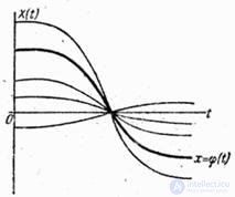
Fig. 16.1.1.

In this case, the abscissa axis also represents one of the possible implementations of the random function implemented when a random variable takes the value 0 (if this value belongs to the number of possible values ​​of ).

As examples of elementary random functions, we give the functions (fig. 16.1.2) and (fig. 16.1.3).

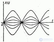
Fig. 16.1.2.

Fig. 16.1.3.

An elementary random function is characterized by the fact that it distinguishes two features of a random function: the entire randomness is concentrated in the coefficient , and the dependence on time - in the usual function .

We define the characteristics of an elementary random function (16.1.3). We have:

,

Where - expectation of a random variable .

If a , expectation of random function is also zero, and the identity is:

.

We know that any random function can be centered, i.e., brought to such a form, when its expectation is zero. Therefore, in the future we will consider only centered elementary random functions for which ; ; .

Define the correlation function of an elementary random function . We have:

,

Where - variance of magnitude .

Above elementary random functions, all sorts of linear transformations are quite simply performed.

For example, let's differentiate the random function (16.1.3). Random value independent of , will be a derivative sign, and we get:

.

Similarly

.

In general, if an elementary random function (16.1.3) is transformed by a linear operator , then with a random factor as independent of , beyond the operator sign, but a non-random function converted by the same operator :

. (16.1.4)

So, if an elementary random function arrives at the input of a linear system, then the task of its transformation is reduced to the simple task of converting a single non-random function. . Hence the idea: if a random form of a general form arrives at the input of a dynamic system, then it can be represented, precisely or approximately, as a sum of elementary random functions and only then subjected to transformation. Such an idea of ​​decomposing a random function into a sum of elementary random functions is the basis of the method of canonical decompositions.

Suppose there is a random function:

. (16.1.5)

Suppose that we were able - precisely or approximately - to represent it as a sum

, (16.1.6)

Where - random variables with mathematical expectations equal to zero; - non-random functions; - expectation function .

We agree to call the representation of a random function in the form (16.1.6) a decomposition of a random function. Random variables will be called the expansion coefficients, and non-random functions - coordinate functions.

Define the reaction of a linear system with an operator on random function given as a decomposition (16.1.6). It is known that a linear system has the so-called property of superposition, consisting in the fact that the response of the system to the sum of several actions is equal to the sum of the reactions of the system to each individual action. Indeed, the system operator Being linear, it can, by definition, be applied to the sum term by term.

Denoting system response to random exposure , we have:

. (16.1.7)

Let's give the expression (16.1.7) a slightly different form. Given the general rule of linear transformation of mathematical expectation, we make sure that

.

Denoting

,

we have:

. (16.1.8)

Expression (16.1.8) is nothing more than a decomposition of a random function on elementary functions. The coefficients of this expansion are the same random variables. , and the expectation and coordinate functions are obtained from the expectation and coordinate functions of the original random function by the same linear transformation to which random function is exposed .

Summarizing, we obtain the following rule for the transformation of a random function given by the decomposition.

If random function given by the decomposition into elementary functions undergoes a linear transformation , the coefficients of decomposition remain unchanged, and the expectation and coordinate functions undergo the same linear transformation .

Thus, the meaning of the decomposition of a random function is reduced to reducing the linear transformation of a random function to the same linear transformation of several non-random functions — expectation and coordinate functions. This allows us to significantly simplify the solution of the problem of finding the characteristics of a random function. compared to the general solution given in 15.7. Indeed, each of the non-random functions , in this case, it is converted only once as opposed to the correlation function which, according to the general rules, is converted twice.