5.6. Position characteristics (expected value, mode, median)

Among the numerical characteristics of random variables, it is necessary, first of all, to note those that characterize the position of the random variable on the numerical axis, i.e. indicate some average, approximate value, around which all possible values ​​of a random variable are grouped.

The average value of a random variable is a certain number, which is, as it were, its “representative” and replaces it with roughly approximate calculations. When we say: “the average lamp operation time is 100 hours” or “the average point of impact is shifted relative to the target 2 m to the right”, we indicate by this a certain numerical characteristic of a random variable describing its location on the numerical axis, i.e. "Position description".

Of the characteristics of a position in probability theory, the most important role is played by the mathematical expectation of a random variable, which is sometimes called simply the average value of a random variable.

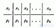
Consider a discrete random variable possible values with probabilities . We need to characterize with some number the position of the values ​​of a random variable on the abscissa axis, taking into account the fact that these values ​​have different probabilities. For this purpose, it is natural to use the so-called "weighted average" of the values each value during averaging, it should be taken into account with a “weight” proportional to the probability of this value. So we calculate the average of the random variable which we denote :

or, considering that ,

. (5.6.1)

This weighted average is called the expectation of a random variable. Thus, we have introduced into consideration one of the most important concepts of probability theory - the concept of mathematical expectation.

The mathematical expectation of a random variable is the sum of the products of all possible values ​​of a random variable on the probability of these values.

Note that in the above formulation, the definition of expectation is valid, strictly speaking, only for discrete random variables; the generalization of this concept to the case of continuous quantities will be given below.

In order to make the concept of mathematical expectation more visual, let us turn to the mechanical interpretation of the distribution of a discrete random variable. Let the points on the abscissa axis with abscissas in which the masses are concentrated respectively , and . Then, obviously, the expectation , defined by the formula (5.6.1), is none other than the abscissa of the center of gravity of a given system of material points.

Mathematical expectation of a random variable connected by a peculiar dependence with the arithmetic average of the observed values ​​of a random variable with a large number of experiments. This dependence is of the same type as the relationship between frequency and probability, namely: with a large number of experiments, the arithmetic mean of the observed values ​​of a random variable approaches (converges in probability) to its mathematical expectation. From the presence of a relationship between frequency and probability, it is possible to deduce as a consequence the presence of a similar relationship between the arithmetic mean and the expectation.

Indeed, consider a discrete random variable characterized by a number of distributions:

Where .

Let produced independent experiments, in each of which the magnitude takes a certain value. Suppose the value appeared times value appeared times in general value appeared time. Obviously

Calculate the arithmetic average of the observed values which, unlike the mathematical expectation we denote :

But there is nothing like the frequency (or statistical probability) of an event ; this frequency can be designated . Then

,

those. the arithmetic mean of the observed values ​​of a random variable is equal to the sum of the products of all possible values ​​of the random variable and the frequencies of these values.

With an increase in the number of experiences frequencies will approach (converge on probability) to the corresponding probabilities . Consequently, the arithmetic average of the observed values ​​of a random variable with an increase in the number of experiments, it will approach (converges in probability) to its expectation .

The connection between the arithmetic mean and the mathematical expectation formulated above is the content of one of the forms of the law of large numbers. Strict proof of this law will be given in Chapter 13.

We already know that all forms of the law of large numbers state the fact of the stability of certain averages with a large number of experiments. Here we are talking about the stability of the arithmetic mean of a number of observations of the same magnitude. With a small number of experiments, the arithmetic mean of their results is random; with a sufficient increase in the number of experiments, it becomes “almost non-random” and, stabilizing, approaches a constant value — the expectation value.

The stability property of averages with a large number of experiments is easy to verify experimentally. For example, weighing any body in the laboratory on exact weights, we obtain a new value each time as a result of weighing; to reduce the error of observation, we weigh the body several times and use the arithmetic average of the obtained values. It is easy to verify that with a further increase in the number of experiments (weighings), the arithmetic average responds to this increase less and less, and with a sufficiently large number of experiments, it practically ceases to change.

The formula (5.6.1) for the expectation value corresponds to the case of a discrete random variable. For continuous value mathematical expectation, of course, is no longer expressed as a sum, but as an integral:

, (5.6.2)

Where - distribution density .

Formula (5.6.2) is obtained from formula (5.6.1), if we replace it with separate values continuously changing parameter x corresponding to probability - element of probability , the final sum is an integral. In the future, we will often use this method of propagating formulas derived for discontinuous quantities in the case of continuous quantities.

In a mechanical interpretation, the expectation of a continuous random variable retains the same meaning — the abscissa of the center of gravity in the case where the mass is distributed along the abscissa axis continuously, with a density . This interpretation often allows one to find the expectation without calculating the integral (5.6.2), from simple mechanical considerations.

Above, we have introduced the designation for expected value . In some cases, when the value enters into formulas as a definite number, it is more convenient to designate it as one letter. In these cases, we will denote the expected value of through :

.

Designations and for the mathematical expectation will be further applied in parallel, depending on the convenience of a particular formula formula. We will also agree, if necessary, to abbreviate the words “mathematical expectation” by the letters m.o.

It should be noted that the most important characteristic of the situation - the expectation - does not exist for all random variables. You can make examples of such random variables for which the expectation does not exist, since the corresponding sum or integral diverge.

Consider, for example, a discontinuous random variable. with a number of distribution:

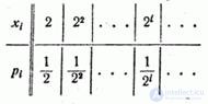
It is not difficult to make sure that i.e. the distribution series makes sense; however the amount in this case it diverges and, therefore, the expected value of does not exist. However, for practice such cases are not of significant interest. Usually, random variables with which we deal have a limited range of possible values ​​and, of course, have a mathematical expectation.

Above, we have given formulas (5.6.1) and (5.6.2) expressing the expectation for a discontinuous and continuous random variable, respectively. .

If the value belongs to the values ​​of the mixed type, its expectation is expressed by the formula of the form:

, (5.6.3)

where the amount applies to all points , in which the distribution function suffers a discontinuity, and the integral - on all areas where the distribution function is continuous.

In addition to the most important of the characteristics of the position — the mathematical expectation — in practice sometimes other characteristics of the position are used, in particular, the mode and median of a random variable.

The mode of a random variable is its most likely value. The term “most likely meaning” strictly applies to discontinuous quantities; for a continuous quantity, the mode is the value at which the probability density is maximum. We agree to denote fashion letter . In fig. 5.6.1 and 5.6.2 shows the mode, respectively, for discontinuous and continuous random variables.

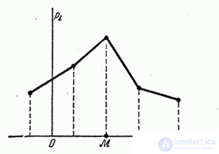
Fig. 5.6.1

Fig. 5.6.2.

If the distribution polygon (distribution curve) has more than one maximum, the distribution is called “polymodal” (Fig. 5.6.3 and 5.6.4).

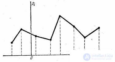
Fig. 5.6.3.

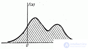
Fig. 5.6.4.

Sometimes there are distributions that have in the middle not a maximum, but a minimum (fig. 5.6.5 and 5.6.6). Such distributions are called "antimodal". An example of an antimodal distribution is the distribution obtained in Example 5, n ° 5.1.

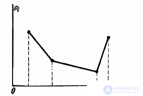
Fig. 5.6.5.

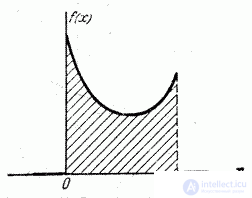
Fig. 5.6.6.

In the general case, the mode and the expectation of a random variable do not coincide. In the particular case when the distribution is symmetric and modal (that is, it has a mode) and there is a mathematical expectation, it coincides with the mode and the center of symmetry of the distribution.

Often, another position characteristic is used — the so-called median of a random variable. This characteristic is usually used only for continuous random variables, although it can be formally defined for a discontinuous value.

The median of a random variable is its value. , for which

,

those. equally likely whether a random variable is smaller or larger . Geometrically, the median is the abscissa of the point at which the area bounded by the distribution curve is divided in half (Fig. 5.6.7).

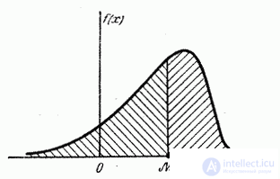
Fig. 5.6.7.

In the case of a symmetric modal distribution, the median coincides with the expectation and mode.