14.2. Estimates for expectation and variance

Let there be a random variable with mathematical expectation and variance ; both parameters are unknown. Above magnitude produced independent experiments that gave results . It is required to find consistent and unbiased estimates for parameters and .

As an estimate for the mathematical expectation, it is natural to propose an arithmetic average of the observed values ​​(previously we denoted it ):

. (14.2.1)

It is easy to verify that this estimate is consistent: according to the law of large numbers, with increasing magnitude converges in probability to . Evaluation is also unbiased since

. (14.2.2)

The variance of this estimate is:

. (14.2.3)

The effectiveness or inefficiency of the assessment depends on the type of distribution law . It can be proved that if distributed according to the normal law, the variance (14.2.3) will be minimally possible, i.e. is effective. For other distribution laws this may not be the case.

We proceed to estimate for variance. . At first glance, the statistical dispersion seems to be the most natural estimate:

, (14.2.4)

Where

. (14.2.5)

Check if this estimate is consistent. Express it through the second initial moment (according to the formula (7.4.6) Chapter 7):

. (14.2.6)

The first term in the right side is the arithmetic mean observed values ​​of random variable ; he converges in probability to . The second term converges in probability to ; the entire quantity (14.2.6) converges in probability to the value

.

This means that the estimate (14.2.4) is consistent.

Check if the score is also unbiased. Substitute in the formula (14.2.6) instead of its expression (14.2.5) and perform the specified actions:

. (14.2.7)

Find the expected value (14.2.7):

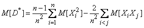. (14.2.8)

Since the variance does not depend on which point you select the origin of coordinates, choose it at the point . Then

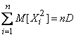; , (14.2.9)

. (14.2.10)

The last equality follows from the fact that the experiments are independent.

Substituting (14.2.9) and (14.2.10) into (14.2.8), we get:

. (14.2.11)

This shows that not an unbiased estimate for : her expectation is not equal and somewhat less. Using the assessment instead of dispersion , we will make some systematic error down. To eliminate this bias, it is enough to introduce an amendment by multiplying the value on . We get:

.

We will choose such a “corrected” statistical variance as an estimate for :

. (14.2.12)

Since the multiplier tends to unit when and score wealthy then estimate will also be wealthy.

In practice, instead of formula (14.2.12), it is often more convenient to apply another, equivalent to it, in which the statistical dispersion is expressed through the second initial moment:

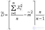. (14.2.13)

For large values naturally both estimates are biased and unbiased - there will be very little difference and the introduction of a correction factor loses its meaning.

Thus, we have arrived at the following rules for processing limited statistical material.

If given values taken in independent experiences random variable with unknown expectation and variance , then to determine these parameters should be used approximate values ​​(estimates):

(14.2.14)