5.1. A number of distribution. Polygon distribution

In the course section on the basic concepts of probability theory, we have already introduced into consideration the extremely important concept of a random variable. Here we will give further development of this concept and indicate the ways in which random variables can be described and characterized.

As already mentioned, a random variable is a quantity that, as a result of experience, can take on a particular value, it is not known beforehand which one. We also agreed to distinguish between random variables of discontinuous (discrete) and continuous types. Possible values ​​of discontinuous values ​​can be pre-listed. Possible values ​​of continuous quantities cannot be pre-listed and continuously fill a certain gap.

Examples of discontinuous random variables:

1) the number of occurrences of the coat of arms with three throws of a coin (possible values ​​are 0, 1, 2, 3);

2) the frequency of the emblem in the same experience (possible values );

3) the number of failed elements in the device, consisting of five elements (possible values ​​are 0, 1, 2, 3, 4, 5);

4) the number of hits in the aircraft, sufficient to disable it (possible values ​​of 1, 2, 3, ..., n, ...);

5) the number of aircraft shot down in air combat (possible values ​​are 0, 1, 2, ..., N, where - the total number of aircraft involved in the battle).

Examples of continuous random variables:

1) the abscissa (ordinate) of the hit point when fired;

2) the distance from the point of impact to the center of the target;

3) height meter error;

4) uptime radio tubes.

Let us further agree on random variables in large letters, and their possible values ​​in corresponding small letters. For example, - number of hits with three shots; possible values: .

Consider a discontinuous random variable with possible values . Each of these values ​​is possible, but not reliable, and the value of X can take each of them with some probability. As a result of the experiment, the value of X will take one of these values, i.e. one of the complete group of incompatible events will occur:

(5.1.1)

Let us denote the probabilities of these events by the letters p with the corresponding indices:

Since incompatible events (5.1.1) form a complete group,

,

those. the sum of the probabilities of all possible values ​​of a random variable is equal to one. This total probability is somehow distributed between individual values. A random variable will be completely described from a probabilistic point of view if we define this distribution, i.e. We indicate exactly what probability each of the events has (5.1.1). By this we establish the so-called law of the distribution of a random variable.

The law of the distribution of a random variable is any relationship that establishes a relationship between the possible values ​​of a random variable and the corresponding probabilities. About a random variable, we will say that it is subject to this distribution law.

Set the form in which the distribution law of a discontinuous random variable can be specified. . The simplest form of setting this law is a table that lists the possible values ​​of a random variable and the corresponding probabilities:

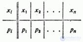
Such a table will be called a series of distribution of a random variable. .

To give the distribution a more visual form, they often resort to its graphic representation: possible values ​​of a random variable are plotted on the abscissa axis, and probabilities of these values ​​are plotted on the ordinate axis. For clarity, the resulting points are connected by straight line segments. Such a figure is called a distribution polygon (Fig. 5.1.1). The distribution polygon, as well as the distribution series, fully characterizes the random variable; It is a form of distribution law.

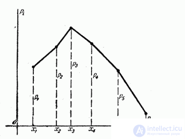
Fig. 5.1.1.

Sometimes the so-called “mechanical” interpretation of a series of distribution is convenient. Imagine that a certain mass equal to unity is distributed along the abscissa axis so that selected points concentrated according to mass . Then the distribution series is interpreted as a system of material points with some masses located on the x-axis.

Let us consider several examples of discontinuous random variables with their distribution laws.

Example 1. One experience is performed in which an event may or may not appear. . Event probability equal to 0.3. Considered a random variable - the number of occurrences in this experience (i.e., the characteristic random variable of the event , taking the value 1 if it appears, and 0 if it does not appear). Construct the distribution series and polygon of the distribution of magnitude .

Decision. Magnitude It has only two values: 0 and 1. The value distribution series has the form:

The distribution polygon is shown in Fig. 5.1.2.

Fig. 5.1.2.

Example 2. The shooter makes three shots at the target. The probability of hitting the target with each shot is 0.4. For each hit the arrow counts 5 points. Build a series of distribution of the number of points knocked out.

Decision. Denote number of points knocked out. Possible values : .

The probability of these values ​​is found by the theorem on the repetition of experiments:

Distribution range has the form:

The distribution polygon is shown in Fig. 5.1.3.

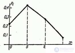
Fig. 5.1.3.

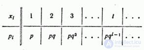
Example 3. The likelihood of an event in one experience is equal . A number of independent experiments are carried out, which continue until the first occurrence of the event. , after which the experiments cease. Random value - the number of experiments made. Build a series of distribution values .

Decision. Possible values : 1, 2, 3, ... (theoretically, they are not limited by anything). To make the value took the value 1, it is necessary that the event happened in the first experience; the probability of this is equal . To make the value took the value 2, it is necessary that in the first experience the event did not appear, and appeared in the second; the probability of this is equal where , etc. Distribution range has the form:

The first five ordinates of the distribution polygon for the case shown in fig. 5.1.4.

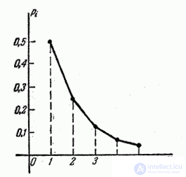
Fig. 5.1.4.

Example 4. The shooter is shooting at the target before the first hit, having 4 rounds ammunition. The probability of hitting each shot is 0.6. Build a number of distribution of ammunition remaining unspent.

Decision. Random value - The number of unused cartridges - has four possible values: 0, 1, 2 and 3. The probabilities of these values ​​are equal, respectively:

Distribution range has the form:

The distribution polygon is shown in fig. 5.1.5.

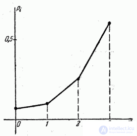
Fig. 5.1.5.

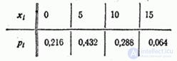
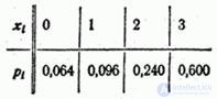
Example 5. A technical device can be used in various conditions and, depending on this, requires adjustment from time to time. With a single use of the device, it may randomly fall into a favorable or unfavorable mode. In a favorable mode, the device withstands three applications without adjustment; before the fourth it has to be regulated. In an unfavorable mode, the device has to be adjusted after the first application. The probability that the device will fall into a favorable mode is 0.7, which is unfavorable, 0.3. Considered a random variable - the number of applications of the device before adjustment. Build its distribution series.

Decision. Random value has three possible values: 1, 2, and 3. The probability that , is equal to the probability that at the first application the device will fall into an unfavorable mode, i.e . To make the value took the value 2, it is necessary that when the device is used for the first time it falls into a favorable mode, and in the second - in an unfavorable one; probability of this . To magnitude took the value 3, it is necessary that the first two times the device falls into a favorable mode (after the third time it will still have to be adjusted). The probability of this is .

Distribution range has the form:

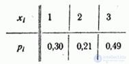
The distribution polygon is shown in fig. 5.1.6.

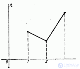
Fig. 5.1.6.