Lecture
In addition to the characteristics of the position - the average, typical values of a random variable - a number of characteristics are used, each of which describes a particular property of the distribution. As such characteristics, so-called moments are most often used.
The concept of moment is widely used in mechanics to describe the mass distribution (static moments, moments of inertia, etc.). The very same methods are used in probability theory to describe the basic properties of the distribution of a random variable. Most often used in practice moments of two types: primary and central.
The initial moment of the s-th order of a discontinuous random variable  called the sum of the form:
 . (5.7.1)
Obviously, this definition coincides with the definition of the initial moment of order s in mechanics, if on the abscissa at the points  concentrated masses
  .
.
For a continuous random variable X, the initial moment of the sth order is the integral
 . (5.7.2)
It is easy to verify that the basic characteristic of the position introduced in the preceding n ° — the mathematical expectation — is nothing but the first initial moment of the random variable. .
Using the expectation sign, you can combine the two formulas (5.7.1) and (5.7.2) into one. Indeed, formulas (5.7.1) and (5.7.2) are completely similar in structure to formulas (5.6.1) and (5.6.2), with the difference that instead of  and
and  cost accordingly
  and
and  . Therefore, we can write a general definition of the initial moment
  th order, valid for both discontinuous and continuous values:
 , (5.7.3)
those. initial moment -th order of random variable called expectation -th degree of this random variable.
Before we define the central moment, we introduce a new concept of a “centered random variable”.
Let there be a random variable with mathematical expectation  . Centered random variable corresponding to magnitude called the deviation of a random variable from her expectation:
 . (5.7.4)
We agree in the following to denote everywhere a centered random variable corresponding to a given random variable with the same letter with the symbol  at the top.
It is easy to verify that the expectation of a centered random variable is zero. Indeed, for a discontinuous value
 ; (5.7.5)
similarly for continuous value.
Centering a random variable is obviously tantamount to transferring the origin to a middle, “central” point, the abscissa of which is equal to the mathematical expectation.
The moments of a centered random variable are called central moments. They are similar to the moments relative to the center of gravity in mechanics.
Thus, the central moment of the order s of a random variable called expectation -th degree of the corresponding centered random variable:
 , (5.7.6)
and for continuous - integral
 . (5.7.8)
In the future, in cases where there is no doubt about the random value of a given moment, for brevity, instead of  and
and  just write
  and
and  .
.
Obviously, for any random variable, the central moment of the first order is zero:
 , (5.7.9)
since the expectation of a centered random variable is always zero.
We derive the relations connecting the central and initial moments of different orders. We will only draw a conclusion for discontinuous values; it is easy to see that exactly the same relations hold for continuous quantities if the final sums are replaced by integrals, and probabilities by probability elements.
Consider the second central point:

Similarly, for the third central moment we get:

Expressions for  etc. can be obtained in a similar way.
Thus, for the central moments of any random variable fair formulas are:
 (5.7.10)
Generally speaking, moments can be considered not only relative to the origin (initial moments) or mathematical expectation (central moments), but also relative to an arbitrary point.  :
:
 . (5.7.11)
However, the central moments have an advantage over all others: the first central moment, as we have seen, is always zero, and the second central moment following it has a minimum value with this frame. Let's prove it. For a discontinuous random variable at  the formula (5.7.11) has the form:
 . (5.7.12)
Convert this expression:

Obviously, this value reaches its minimum when  i.e. when the moment is taken relative to the point .
Of all the moments, the first initial moment (mathematical expectation) is most often used as the characteristics of a random variable.  and the second central point
  .
.
The second central moment is called the variance of the random variable. In view of the extreme importance of this characteristic, among other things, we introduce a special designation for it.  :
:
 .
.
According to the definition of the central moment
 , (5.7.13)
those. the variance of the random variable X is the mathematical expectation of the square of the corresponding centered value.
Replacing the value in expression (5.7.13)  by its expression, we also have:
 . (5.7.14)
For the direct calculation of the variance are the formulas:
 , (5.7.15)
 (5.7.16)
- respectively for discontinuous and continuous values.
Variance of a random variable is a characteristic of dispersion, the dispersion of values of a random variable around its expectation. The word "dispersion" itself means "dispersion."
If we turn to the mechanical interpretation of the distribution, then the variance is nothing but the moment of inertia of a given mass distribution relative to the center of gravity (mathematical expectation).
The variance of the random variable has the dimension of the square of the random variable; for visual dispersion characteristics, it is more convenient to use a quantity whose dimension coincides with the dimension of a random variable. For this, the square root is extracted from the dispersion. The resulting value is called the standard deviation (otherwise - "standard") of a random variable. . Standard deviation will be denoted by  :
:
 , (5.7.17)
To simplify the records, we will often use the abbreviated notation for the standard deviation and variance:  and
and  . In the case when there is no doubt what random value these characteristics belong to, we will sometimes omit the xy icon and and just write
  and
and  . The words "standard deviation" will sometimes be abbreviated to replace the letters with.
In practice, a formula is often used expressing the variance of a random variable through its second initial moment (the second of formulas (5.7.10)). In the new notation, it will look like:
 . (5.7.18)
Expected value and variance (or mean square deviation ) - the most frequently used characteristics of a random variable. They characterize the most important features of the distribution: its position and degree of dispersion. For a more detailed description of the distribution, higher order moments are used.
The third central moment serves to characterize the asymmetry (or "skewness") of the distribution. If the distribution is symmetrical with respect to the expectation (or, in a mechanical interpretation, the mass is distributed symmetrically with respect to the center of gravity), then all moments of an odd order (if they exist) are equal to zero. Indeed, in sum

with relatively symmetrical distribution law and odd each positive term corresponds to a negative term equal to it in absolute value, so that the whole sum is zero. The same is obviously true for the integral
 ,
,
which is zero, as an integral in the symmetric range of an odd function.
It is therefore natural to choose one of the odd moments as a characteristic of the asymmetry of the distribution. The simplest of them is the third central moment. It has the dimension of a cube of a random variable: in order to obtain a dimensionless characteristic, the third moment  divided by the cube of the standard deviation. The value obtained is called the “asymmetry coefficient” or simply “asymmetry”; we denote it
  :
:
 . (5.7.19)
In fig. 5.7.1 shows two asymmetric distributions; one of them (curve I) has a positive asymmetry (  ); other (curve II) - negative (
  ).
).
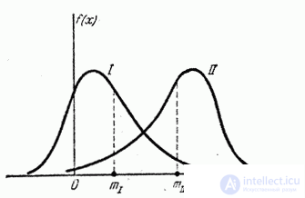
Fig. 5.7.1
The fourth central moment serves to characterize the so-called "coolness", i.e. sharpness or flatness distribution. These properties of the distribution are described by the so-called kurtosis. Excesses of random variables called magnitude
 . (5.7.20)
The number 3 is subtracted from the relationship  because for the very important and widespread in nature normal distribution law (with which we will get acquainted in detail later)
  . Thus, for a normal distribution, kurtosis is zero; curves, more pointed than normal, have positive kurtosis; curves more flat-topped - negative kurtosis.
In fig. 5.7.2 are presented: normal distribution (curve I), distribution with positive kurtosis (curve II) and distribution with negative kurtosis (curve III).
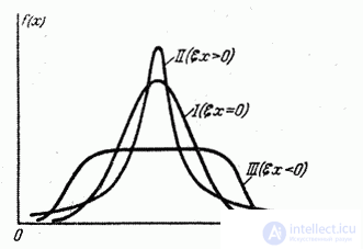
Fig. 5.7.2
In addition to the above initial and central moments, in practice sometimes used the so-called absolute moments (initial and central), defined by the formulas
 ;
;  .
.
Obviously, the absolute moments of even orders coincide with the usual moments.
Of the absolute moments, the first absolute central moment is most often used.
 , (5.7.21)
called average arithmetic deviation. Along with variance and standard deviation, the arithmetic average deviation is sometimes used as a scattering characteristic.
Mathematical expectation, mode, median, initial and central moments and, in particular, variance, standard deviation, asymmetry and kurtosis are the most commonly used numerical characteristics of random variables. In many problems of practice, a complete characteristic of a random variable — the law of distribution — is either not needed or cannot be obtained. In these cases, limited to an approximate description of a random variable with help. Numerical characteristics, each of which expresses some characteristic property of the distribution.
Very often, numerical characteristics are used to approximate the replacement of one distribution by another, and they usually strive to make this replacement so that several important points remain unchanged.
Example 1. One experience is performed, as a result of which an event may or may not appear.  whose probability is equal
  . Considered a random variable - the number of occurrences (characteristic random variable of event ). Determine its characteristics: expectation, variance, standard deviation.
Decision. The series of distribution of the value is:
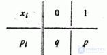
Where  - probability of non-occurrence .
By the formula (5.6.1) we find the expected value of :
 .
.
Variance of magnitude determined by the formula (5.7.15):
 ,
,
from where
 .
.
(We offer the reader to get the same result, expressing the variance through the second initial moment).
Example 2. Three independent target shots are made; the probability of hitting each shot is 0.4. random value - number of hits. Determine the magnitude characteristics - expectation, variance, ko, asymmetry.
Decision. Distribution range has the form:
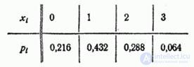
We calculate the numerical characteristics of the value :

Note that the same characteristics could be computed much simpler with the help of theorems on the numerical characteristics of functions (see Chapter 10).
Example 3. A series of independent experiments are made before the first occurrence of an event. (see example 3 n ° 5.1). Event probability in each experience is equal . Find the expectation, variance and sc. the number of experiments that will be made.
Decision. Distribution range has the form:
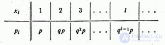
Expectation value expressed by the sum of a row
 .
.
Нетрудно видеть, что ряд, стоящий в скобках, представляет собой результат дифференцирования геометрической прогрессии:

Consequently,

from where
 .
.
Для определения дисперсии величины Х вычислим сначала её второй начальный момент:
 .
.
Для вычисления ряда, стоящего в скобках, умножим на q ряд:

We get:

Дифференцируя этот ряд по  , we have:

Умножая на  , we get:

По формуле (5.7.18) выразим дисперсию:

from where

Пример 4. Непрерывная случайная величина subject to the distribution law with a density of:

(рис. 5.7.3).
Найти коэффициент . Определить м.о., дисперсию, с.к.о., асимметрию, эксцесс величины .
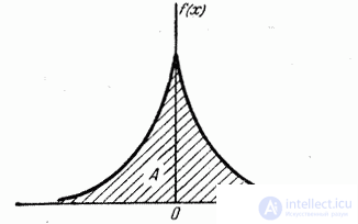
Fig. 5.7.3.
Decision. For determining воспользуемся свойством плотности распределения:

from here  .
.
Так как функция  нечетная, то м.о. величины равно нулю:
 .
.
Дисперсия и с.к.о. равны, соответственно:
 .
.
Так как распределение симметрично, то  .
.
Для вычисления эксцесса находим  :
:

from where
 .
.
Пример 5. Случайная величина подчинена закону распределения, плотность которого задана графически на рис. 5.7.4.
Write an expression for the density of distribution. Найти м.о., дисперсию, с.к.о. и асимметрию распределения.

Fig. 5.7.4.
Decision. Выражение плотности распределения имеет вид:

Пользуясь свойством плотности распределения, находим  .
.
Математическое ожидание величины :

Дисперсию найдем через второй начальный момент:

from here

Третий начальный момент равен

Пользуясь третьей из формул (5.7.10), выражающей через начальные моменты, имеем:

from where


Comments
To leave a comment
Probability theory. Mathematical Statistics and Stochastic Analysis
Terms: Probability theory. Mathematical Statistics and Stochastic Analysis