Lecture
In solving various problems associated with random phenomena, modern probability theory makes extensive use of the apparatus of random variables. In order to use this apparatus, it is necessary to know the laws of the distribution of random majesty appearing in the problem. Generally speaking, these laws can be determined from experience, but usually experience whose goal is to determine the law of distribution of a random variable or a system of random variables (especially in the field of military equipment) turns out to be both difficult and expensive. Naturally, the problem arises - to reduce the amount of experiment to a minimum and make a judgment about the laws of distribution of random variables indirectly, based on the already known laws of distribution of other random variables. Such indirect methods of research of random variables play a very large role in the theory of probability. In this case, the random variable that is usually of interest to us is represented as a function of other random variables; knowing the laws of the distribution of arguments, it is often possible to establish the law of distribution of a function. We will meet with a number of tasks of this type in the future (see Chapter 12).
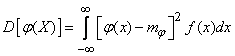
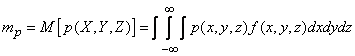
However, in practice, there are often cases when there is no special need to fully determine the distribution law of the function of random variables, and it suffices only to indicate its numerical characteristics: expectation, variance, sometimes some of the highest moments. In addition, very often the very laws of the distribution of arguments are not well known. In this connection, the problem often arises of determining only numerical characteristics of functions of random variables.
Consider the following problem: a random variable  there is a function of several random variables
  :
:
 .
.
Let us know the law of distribution of the system of arguments.  ; required to find the numerical characteristics of the value in the first place - the expectation and variance.
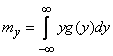
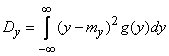
Imagine that we managed in one way or another to find the distribution law  magnitudes . Then the problem of determining numerical characteristics becomes trivial; they are according to the formulas:
 ;
;
etc.
However, the very task of finding the distribution law magnitudes often turns out to be quite complicated. In addition, to solve the problem posed by us, finding the distribution law for the quantity as such, it is not at all necessary: to find only numerical characteristics of a quantity there is no need to know its distribution law; enough to know the distribution of arguments . Moreover, in some cases, in order to find the numerical characteristics of a function, it is not even necessary to know the distribution law of its arguments; it is enough to know only some numerical characteristics of the arguments.
Thus, the problem arises of determining the numerical characteristics of functions of random variables in addition to the laws of distribution of these functions.
Consider the problem of determining the numerical characteristics of a function for a given distribution of arguments. Let's start with the simplest case - the function of one argument - and set the following task.
There is a random variable  with a given distribution law; another random variable associated with functional dependence:
 .
.
Required without finding the distribution law of magnitude , determine its expectation:
 . (10.1.1)
Consider first the case when there is a discontinuous random variable with a series of distribution:
|
|
|
|
|
|
|
|
|
|
Write down possible values and the probabilities of these values:
|
|
|
|
|
|
|
|
|
|
(10.1.2)
Table (10.1.2) is not strictly a series of distribution of , since in general some of the values
 (10.1.3)
may coincide with each other; moreover, these values in the upper column of the table (10.1.2) do not necessarily go in ascending order. In order to move from a table (10.1.2) to a genuine series of distribution of , it would be necessary to arrange the values (10.1.3) in ascending order, combine the columns corresponding to the equal values and add up the corresponding probabilities. But in this case we are not interested in the distribution law as such; for our purposes — determining the expectation — it is enough to have such an “unordered” form of the distribution series as (10.1.2). Expectation value can be determined by the formula
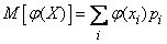 (10.1.4)
Obviously the magnitude , determined by the formula (10.1.4), cannot change due to the fact that under the sign of the sum some members will be combined in advance, and the order of the members will be changed.
The formula (10.1.4) for the mathematical expectation of a function is not explicitly contained in the distribution law of the function itself, but only the distribution law of the argument. Thus, to determine the mathematical expectation of a function, it is not at all necessary to know the distribution law of this function, but it is sufficient to know the distribution law of the argument.
Replacing in the formula (10.1.4) the sum with the integral, and the probability  - an element of probability, we obtain a similar formula for a continuous random variable:
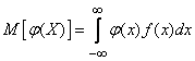 . (10.1.5)
Where  - distribution density .
Similarly, the expectation of a function can be determined  from two random arguments and . For discontinuous values
 , (10.1.6)
Where  - the probability that the system
  will take values
  .
.
For continuous values
 , (10.1.7)
Where  - system distribution density .
The mathematical expectation of a function is determined in exactly the same way from an arbitrary number of random arguments. We present the corresponding formula only for continuous values:

 (10.1.8)
Where  - system distribution density .
Formulas of the type (10.1.8) are very often encountered in the practical application of probability theory when it comes to averaging some values depending on a number of random arguments.
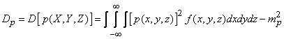
Thus, the expectation of a function of any number of random arguments can be found in addition to the law of distribution of the function. Similarly, other numerical characteristics of the function can be found - moments of different orders. Since each moment is the mathematical expectation of a certain function of the random variable under study, the calculation of any moment can be carried out by methods completely similar to the above. Here we present calculation formulas only for variance, and only for the case of continuous random arguments.
The variance of a function of one random argument is expressed by the formula
 , (10.1.9)
Where  - expectation function
  ; - distribution density .
The variance of the function of two arguments is expressed similarly:
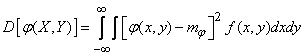 (10.1.10)
Where  - expectation function ; - system distribution density .
Finally, in the case of an arbitrary number of arguments, in a similar notation:

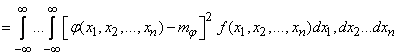 . (10.1.11)
Note that often when calculating the variance it is convenient to use the ratio between the initial and central moments of the second order (see Chapter 5) and write:
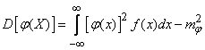 ; (10.1.12)
 ; (10.1.13)
 . (10.1.14)
Formulas (10.1.12) - (10.1.14) can be recommended when they do not lead to differences of close numbers, i.e. when relatively small.
Let us consider several examples illustrating the application of the above methods for solving practical problems.
Example 1. A length segment is specified on a plane.  (fig. 10.1.1), rotating randomly so that all directions are equally likely. The segment is projected on a fixed axis.
  . Determine the average length of the projection of the segment.
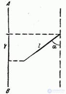
Fig. 10.1.1
Decision. The length of the projection is:
 ,
,
where is the angle  - random variable distributed with uniform density on the plot
  .
.
By the formula (10.1.5) we have:
 .
.
Example 2. The elongated fragment of the projectile, which can be schematically depicted a segment of length , flies, rotating around the center of mass in such a way that all its orientations in space are equally likely. On its way, the fragment meets a flat screen, perpendicular to the direction of its movement, and leaves a hole in it. Find the expectation of the length of this hole.
Decision. First of all, we give the mathematical formulation of the assertion that “all orientations of a fragment in space are equally probable.” Cut direction we will characterize the unit vector  (fig. 10.1.2).
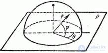
Fig. 10.1.2
Vector direction in a spherical coordinate system associated with a plane  on which the design is made, is determined by two angles:
  lying in a plane and angle
  lying in a plane perpendicular to . With equal probability of all directions of the vector all positions of its end on the surface of a sphere of a single radius
  must have the same probability density; therefore, the element of probability
 ,
,
Where  - density of distribution of angles
  , must be proportional to the elemental area
  on the sphere ; this elementary area is equal
 ,
,
from where
 ;
;  ,
,
Where  - coefficient of proportionality.
Coefficient value we find from the relation
 ,
,
from where
 .
.
Thus, the density of the distribution of angles expressed by the formula
 at
at  (10.1.15)
Design the segment na plane ; projection length is equal to:
 .
.
Considering as a function of two arguments and and applying the formula (10.1.7), we obtain:
 .
.
Thus, the average length of a hole left by a fragment in the screen is equal to  shard lengths
Example 3. Flat area figure  randomly rotates in space so that all orientations of this figure are equally likely. Find the average projected area of the figure on a fixed plane (fig. 10.1.3).
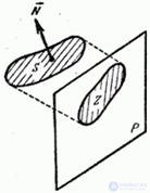
Fig. 10.1.3
Decision. Direction of the plane of the figure in space we will characterize the direction of the normal  to this plane. With a plane bind the same spherical coordinate system as in the previous example. Normal direction to the site characterized by random angles and distributed with density (10.1.5). Square
  figure projections on the plane equals
 ,
,
and the average projection area
 .
.
Thus, the average projected area of an arbitrarily oriented flat figure on a fixed plane is equal to half the area of this figure.
Example 4. In the process of tracking by a radar behind a certain object, the spot depicting the object is kept all the time within the limits of the screen. The screen is a circle  radius
  . The spot occupies a random position on the screen with a constant probability density. Find the average distance from the spot to the center of the screen.
Decision. Denoting the distance  we have
  where
where  - coordinates of the spot;
  within a circle and is zero beyond. Applying the formula (10.1.7) and passing to the polar coordinates in the integral, we have:
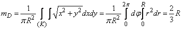 .
.
Example 5. Reliability (probability of failure-free operation) of a technical device is a certain function.  three parameters characterizing the operation of the regulator. Options
  are random variables with a known distribution density
  . Find the average value (mathematical expectation) of the reliability of the device and the standard deviation characterizing its stability.
Decision. Device reliability there is a function of three random variables (parameters) . Its average value (mathematical expectation) can be found by the formula (10.1.8):
 . (10.1.16)
According to the formula (10.1.14) we have:
 ,
,
 .
.
Formula (10.1.16), expressing the average (full) probability of failure-free operation of the device, taking into account the random greatness, on which this probability depends in each particular case, is a special case of the so-called integral formula of total probability, which generalizes the usual total probability formula to the case of infinite (uncountable) number of hypotheses.
We derive here this formula in general.
Suppose that an experience in which an event of interest may or may not appear , proceeds in random, previously unknown conditions. Let these conditions be characterized by continuous random variables.
, (10.1.17)
distribution density of which
.
Probability  occurrence of an event there is a certain function of random variables (10.1.17):
 . (10.1.18)
We need to find the mean value of this probability or, in other words, the total probability of an event. :
 .
.
Applying formula (10.1.8) for the mathematical expectation of a function, we find:
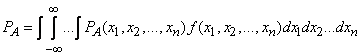 . (10.1.19)
Формула (10.1.19) называется интегральной формулой полной вероятности. Нетрудно заметить, что по своей структуре она сходна с формулой полной вероятности, если заменить дискретный ряд гипотез непрерывной гаммой, сумму - интегралом, вероятность гипотезы - элементом вероятности:
 ,
,
а условную вероятность события при данной гипотезе - условной вероятностью события при фиксированных значениях случайных величин:
 .
.
Не менее часто, чем интегральной формулой полной вероятности пользуются интегральной формулой полного математического ожидания. Эта формула выражает среднее (полное) математическое ожидание случайной величины , значение которой принимается в опыте, условия которого заранее неизвестны (случайны). Если эти условия характеризуются непрерывными случайными величинами
with distribution density
,
and the expectation of a quantity is a function of :
 ,
,
then the total expected value calculated by the formula
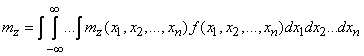 (10.1.20)
which is called the integral total expectation formula.
Example 6. The mathematical expectation of the distance at which an object will be detected using four radar stations depends on some of the technical parameters of these stations:
 ,
,
which are independent random variables with distribution density
 .
.
For fixed parameters, the  expectation of the detection range is
 .
.
Find the average (full) expectation of the detection range.
Decision. According to the formula (10.1.20) we have:
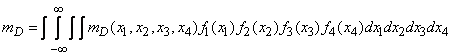 .
.


Comments
To leave a comment
Probability theory. Mathematical Statistics and Stochastic Analysis
Terms: Probability theory. Mathematical Statistics and Stochastic Analysis