10.2. Numerical Characteristics Theorems

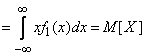
In the previous We have given a number of formulas that allow us to find the numerical characteristics of functions when the laws of the distribution of arguments are known. However, in many cases, to find the numerical characteristics of functions, it is not even necessary to know the distribution laws of the arguments, it is sufficient to know only some of their numerical characteristics; at the same time, we generally do without any laws of distribution. Determining the numerical characteristics of functions by given numerical characteristics of the arguments is widely used in probability theory and can significantly simplify the solution of a number of problems. For the most part, such simplified methods relate to linear functions; however, some elementary nonlinear functions also allow a similar approach.

Present we present a series of theorems on the numerical characteristics of functions, which in their totality represent a very simple apparatus for calculating these characteristics, applicable in a wide range of conditions.

1. The mathematical expectation of non-random values

If a - non-random value, then

.

The formulated property is fairly obvious; you can prove it by considering a non-random value as a particular type of random, with one possible value with a probability of one; then according to the general formula for the expectation:

.

2. Non-random variance

If a - non-random value, then

.

Evidence. By definition dispersion

.

3. Making the non-random value a sign of the expectation

If a - non-random value, and - random, then

, (10.2.1)

that is, a nonrandom value can be taken beyond the sign of the expectation.

Evidence.

a) For discontinuous quantities

.

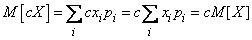b) For continuous values

.

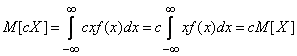4. The introduction of non-random values ​​for the sign of the variance and standard deviation

If a - non-random value, and - random, then

, (10.2.2)

that is, it is possible to take a nonrandom value by the sign of the dispersion, squaring it.

Evidence. By definition dispersion

.

The investigation

,

that is, a nonrandom value can be taken beyond the sign of the standard deviation of its absolute value. The proof will be obtained by extracting the square root from formula (10.2.2) and taking into account that sk. - substantially positive value.

5. The mathematical expectation of the sum of random variables

Let us prove that for any two random variables and

, (10.2.3)

that is, the expectation of the sum of two random variables is equal to the sum of their expectation values.

This property is known as the theorem of addition of mathematical expectations.

Evidence.

a) Let - system of discontinuous random variables. Apply to the sum of random variables the general formula (10.1.6) for the mathematical expectation of a function of two arguments:

.

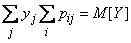
Ho is nothing but the total probability that the magnitude will take value :

;

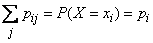Consequently,

.

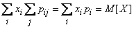Similarly, we prove that

,

and the theorem is proved.

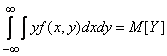
b) Let - system of continuous random variables. According to the formula (10.1.7)

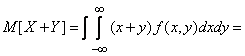
. (10.2.4)

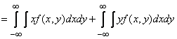
Convert the first of the integrals (10.2.4):

;

similarly

,

and the theorem is proved.

It should be specially noted that the theorem of addition of mathematical expectations is valid for any random variables, both dependent and independent.

The theorem of addition of mathematical expectations is generalized to an arbitrary number of terms:

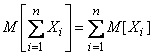, (10.2.5)

that is, the expectation of the sum of several random variables is equal to the sum of their expectation values.

For the proof, it suffices to apply the method of complete induction.

6. Mathematical expectation of a linear function

Consider a linear function of several random arguments. :

,

Where - non-random coefficients. Prove that

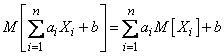, (10.2.6)

that is, the expectation of a linear function is equal to the same linear function of the expectation of the arguments.

Evidence. Using the addition theorem and the rule of making a nonrandom value for the sign of M. o., we obtain:

.

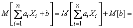
7. Disp of these sums of random variables

The variance of the sum of two random variables is equal to the sum of their variances plus the doubled correlation moment:

. (10.2.7)

Evidence. Denote

. (10.2.8)

By the theorem of addition of mathematical expectations

. (10.2.9)

Let's move from random variables to the corresponding centered values . Subtracting term by term from equality (10.2.8) equality (10.2.9), we have:

.

By definition dispersion

,

Q.E.D.

Formula (10.2.7) for the variance of the sum can be generalized to any number of terms:

, (10.2.10)

Where - correlation moment of magnitudes , sign a sum means that the summation applies to all possible pairwise combinations of random variables .

The proof is similar to the previous one and follows from the formula for the square of a polynomial.

Formula (10.2.10) can be written in another form:

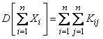, (10.2.11)

where the double sum applies to all elements of the correlation matrix of the system of values containing both correlation moments and variances.

If all random variables included in the system are uncorrelated (i.e. at ), the formula (10.2.10) takes the form:

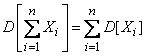(10.2.12)

that is, the variance of the sum of uncorrelated random variables is equal to the sum of the variances of the terms.

This position is known as the theorem of addition of variances.

8. Dispersion of a linear function

Consider a linear function of several random variables.

,

Where - non-random values.

We prove that the variance of this linear function is expressed by the formula

, (10.2.13)

Where - correlation moment of magnitudes , .

Evidence. We introduce the notation:

.

Then

. (10.2.14)

Applying to the right side of the expression (10.2.14) the formula (10.2.10) for the variance of the sum and taking into account that , we get:

, (10.2.15)

Where - correlation moment of magnitudes :

.

Calculate this moment. We have:

;

similarly

.

From here

.

Substituting this expression in (10.2.15), we arrive at the formula (10.2.13).

In the particular case when all values uncorrelated, the formula (10.2.13) takes the form:

, (10.2.16)

that is, the variance of a linear function of uncorrelated random variables is equal to the sum of the products of the squares of the coefficients on the variance of the corresponding arguments.

9. The mathematical expectation of the product of random variables.

The expectation of the product of two random variables is equal to the product of their expectation plus the correlation moment:

. (10.2.17)

Evidence. We will proceed from the definition of the correlation moment:

,

Where

; .

Let us transform this expression using the properties of the expectation:

,

which is obviously equivalent to the formula (10.2.17).

If random values uncorrelated , the formula (10.2.17) takes the form:

, (10.2.18)

that is, the mathematical expectation of the product of two uncorrelated random variables is equal to the product of their mathematical expectation.

This position is known as the theorem of multiplying mathematical expectations.

Formula (10.2.17) is nothing but the expression of the second mixed central moment of the system in terms of the second mixed initial moment and mathematical expectations:

. (10.2.19)

This expression is often used in practice when calculating the correlation moment in the same way as for one random variable the variance is often calculated through the second initial moment and the expectation.

The theorem of multiplying mathematical expectations is generalized to an arbitrary number of factors, only in this case it is not enough for its application that the values ​​be uncorrelated, but it is required that some higher mixed moments, the number of which depends on the number of terms in the work, vanish. These conditions are certainly fulfilled with the independence of the random variables in the product. In this case

(10.2.20)

that is, the expectation of the product of independent random variables is equal to the product of their expectation.

This position is easily proved by the method of complete induction.

10. Dispersion of a product of independent random variables.

Let us prove that for independent quantities

. (10.2.21)

Evidence. Denote . By definition dispersion

.

As magnitudes independent and

.

With independent magnitudes also independent; Consequently,

,

and

. (10.2.22)

But there is nothing like the second initial moment of magnitude , and, therefore, is expressed through the variance:

;

similarly

.

Substituting these expressions into formula (10.2.22) and citing similar terms, we arrive at formula (10.2.21).

In the case when centered random variables are multiplied (values ​​with mathematical expectation equal to zero), the formula (10.2.21) takes the form:

(10.2.23)

that is, the variance of the product of independent centered random variables is equal to the product of their variances.

11. Highest moments of the sum of random variables.

In some cases, it is necessary to calculate the highest moments of the sum of independent random variables. Let us prove some related relations.

1) If quantities independent then

. (10.2.24)

Evidence.

,

whence according to the theorem of multiplication of mathematical expectations

.

But the first central point for any value is zero; two middle terms vanish, and the formula (10.2.24) is proved.

The ratio (10.2.24) by the induction method is easily generalized to an arbitrary number of independent terms:

. (10.2.25)

2) The fourth central moment of the sum of two independent random variables is expressed by the formula

. (10.2.26)

Where - dispersion of values and .

The proof is completely analogous to the previous one.

Using the complete induction method, it is easy to prove a generalization of formula (10.2.26) to an arbitrary number of independent terms:

. (10.2.27)

Similar relations, if necessary, can be easily derived for moments of higher orders.

12. Addition of uncorrelated random vectors.

Consider on the plane two uncorrelated random vectors: vector with components and vector with components (fig. 10.2.1).

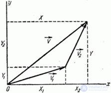
Fig. 10.2.1

Consider their vector sum:

,

i.e. a vector with components:

,

.

Required to determine the numerical characteristics of a random vector - mathematical expectations , variance and correlation moment of the components: .

By the theorem of addition of mathematical expectations:

;

.

According to the theorem of addition of variances

;

.

Let us prove that the correlation moments also add up:

, (10.2.28)

Where - correlation moments of the components of each of the vectors and .

Evidence. By definition, the correlation moment:

. (10.2.29)

Since vectors are and некоррелированны, то два средних члена в формуле (10.2.29) равны нулю; два оставшихся члена представляют собой and ; формула (10.2.28) доказана.

Формулу (10.2.28) иногда называют «теоремой сложения корреляционных моментов».

Теорема легко обобщается на произвольное число слагаемых. Если имеется две некоррелированные системы случайных величин, т. е. два -мерных случайных вектора:

with components ,

with components ,

то их векторная сумма

имеет корреляционную матрицу, элементы которой получаются суммированием элементов корреляционных матриц слагаемых:

, (10.2.30)

Where обозначают соответственно корреляционные моменты величин ; ; .

Формула (10.2.30) справедлива как при , так и при . Действительно, составляющие вектора are equal:

По теореме сложения дисперсий

,

или в других обозначениях

.

По теореме сложения корреляционных моментов при

.

В математике суммой двух матриц называется матрица, элементы которой получены сложением соответствующих элементов этих матриц. Пользуясь этой терминологией, можно сказать, что корреляционная матрица суммы двух некоррелированных случайных векторов равна сумме корреляционных матриц слагаемых:

. (10.2.31)

Это правило по аналогии с предыдущими можно назвать «теоремой сложения корреляционных матриц».