Lecture
I am glad when, in addition to new constellations, there is something similar to dependence on the diagram. In this case, we build a model that well explains the relationship between the two variables. But the researcher must understand not only how to work with the data, but also what kind of real-world story lies behind it. Otherwise, it's easy to make a mistake. I'll tell you about the Simpson Paradox, one of the most dangerous examples of deceptive data that can turn a connection upside down.
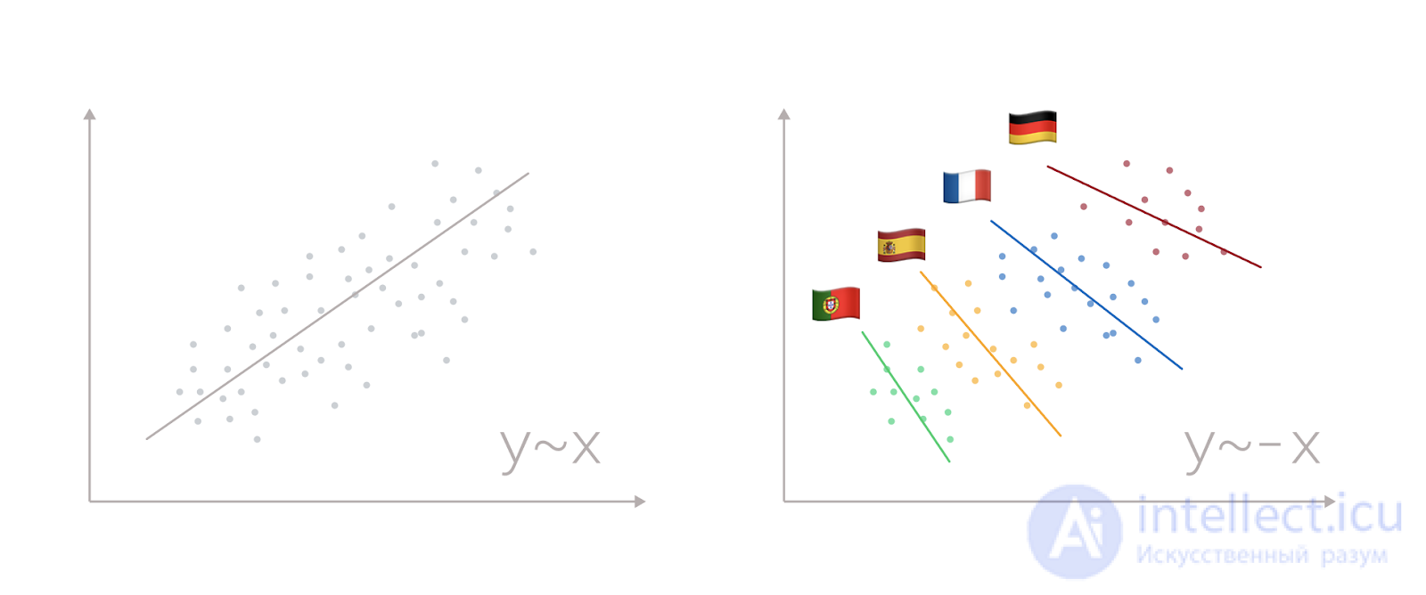
Let's look at the two conditional variables X and Y. Having built the diagram, we will see a cloud clearly stretched from the lower left corner to the upper right corner, as in the picture above. Linear regression fits perfectly into such a picture, which, with a relatively low error, will help us predict values: the more X, the more Y. The task is completed. At first sight.
A more experienced colleague will recommend that we add a breakdown by cohorts to the diagram: for example, by country. Following his advice, we will see that there really is a connection, but it is diametrically opposite - within a single country, the more X, the less Y.
This is the Simpson paradox: a phenomenon in which the combination of several groups of data with the same directional dependence leads to changing direction to the opposite.
The most famous example of the Simpson Paradox in the real world is the sex discrimination confusion of admission to the University of Berkeley in 1973. There is a rumor among researchers that the university was even tried, but there is no convincing evidence of a trial on the Internet.
This is how the university admission statistics for 1973 looks like:
| Floor | Applications | Received |
| Men | 8442 | 3738 (44%) |
| Women | 4321 | 1494 (35%) |
The difference is significant. Too big to be random.
However, when the data is disaggregated by faculty, the picture changes. The researchers found that the reason for the difference was that women applied for more competitive destinations. In addition, it was found that 6 out of 85 faculties discriminated in favor of women, and only 4 did not.
The difference is solely due to differences in sample sizes and competition sizes between faculties. I will show it by the example of two faculties.
| Faculty | Floor | Applications | Received |
| A | Men | 400 | 200 (50%) |
| A | Women | 200 | 100 (50%) |
| B | Men | 150 | 50 (33%) |
| B | Women | 450 | 150 (33%) |
| Total | Men | 550 | 250 (45%) |
| Total | Women | 650 | 250 (38%) |
Both faculties accept the same proportion of women and men. However, since the absolute number of men was higher in the faculty with a higher acceptance rate, if we combine the data, the overall male enrollment rate is higher.
Imagine doing an A / B experiment to boost your landing page's conversions. The experiment runs for two days, but on the first day the visitor distributor broke down and option B received more visitors. On the second day, this problem was fixed. The result is the following figures:
| A | B | |||
| Visitors | Conversions | Visitors | Conversions | |
| Day 1 | 400 | 30 (7.5%) | 2000 | 140 (7%) |
| Day 2 | 1000 | 60 (6.0%) | 1000 | 55 (5.5%) |
| Total | 1400 | 90 (6.4%) | 3000 | 195 (6.5%) |
Option A had a higher conversion rate on every single day, but option B wins overall, because option B had more traffic on the higher converting day. In this example, an inexperienced researcher will roll out option B for all traffic, while in fact, the conversion will increase if he uses option A.
Each site has a page that motivates people to buy more than others. Suppose we create a visitor scoring system and select factors for it. We have an About Product page and we assume that visiting it increases the likelihood of conversion. Let's look at the data.
| Visited the page | ||
| Conversion | Not | Yes |
| Not | 4000 | 4800 |
| Yes | 400 | 320 |
| Conversion rate | nine% | 6% |
At first glance, everything is obvious - the conversion for visitors to the page is as much as 3 pp less, which means that the page reduces the likelihood of conversion. But if we break the data down into the two most important cohorts in internet marketing, desktop and mobile, we see that in fact, in each of them, the likelihood of conversion increases with a visit to the page.
| Mobile | Desktop | |||
| Visited the page | Visited the page | |||
| Conversion | Not | Yes | Not | Yes |
| Not | 1600 | 4200 | 2400 | 600 |
| Yes | 40 | 180 | 360 | 140 |
| Conversion rate | 2% | 4% | 13% | nineteen% |
We assumed that the visit to the page affects the conversion. In practice, a third variable intervened - the user's platform. Due to the fact that it affects not only the conversion, but also the likelihood of visiting the page, in an aggregated state, it distorted the data in such a way that led us to conclusions that were opposite to the real behavior of users.

In data analysis, you need to understand what the story lies behind them: what is happening in the real world, how it was measured and translated into data. So the data scientist in the marketing department needs to know the basics of marketing, and in the oil and gas industry something about mining. This will help to avoid a lot of potential errors, not the least of which is the aggregation error caused by the Simpson paradox.
The following characteristics of the data usually lead to the appearance of the Simpson Paradox:
Each case requires an individual approach. Considering that all data must always be split into cohorts is also a wrong approach, because often it is aggregated data that allows you to build the most accurate model. In addition, any data can be broken down to get the relationship that we would like to get. True, this will not have any practical application - the cohorts must be justified.
For internet marketing, one of the most important takeaways is the need to test the splitter correctly in A / B experiments. The user groups in each test case should be approximately the same. It's not only about the total number of users, but also about their structure. If problems are suspected, cohorts should be tested first for the following characteristics:

Comments
To leave a comment
Probability theory. Mathematical Statistics and Stochastic Analysis
Terms: Probability theory. Mathematical Statistics and Stochastic Analysis