Lecture
Consider two independent random variables.  and
and  , subject to normal laws:
 , (12.6.1)
 . (12.6.2)
It is required to produce a composition of these laws, i.e., to find the law of distribution of magnitude:
 .
.
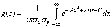
We apply the general formula (12.5.3) to the composition of the laws of distribution:

 . (12.6.3)
If we expand the brackets in the exponent of the integrand function and give similar terms, we get:
 ,
,
Where
 ;
;
 ;
;
 .
.
Substituting these expressions into the formula we have already encountered (9.1.3):
 , (12.6.4)
after transformation we get:
 , (12.6.5)
and this is nothing but a normal law with a center of dispersion
 (12.6.6)
and standard deviation
 . (12.6.7)
Moreover, the conclusion can be made much simpler with the help of the following qualitative considerations.
Without opening the brackets and not making the transformations in the integrand function (12.6.3), we immediately conclude that the exponent is a square trinomial with respect to  kind of
 ,
,
where is the coefficient  magnitude
  not included at all
  included in the first degree, and in the coefficient
  - squared. With this in mind and applying the formula (12.6.4), we conclude that
  there is an exponential function, the exponent of which is a square triple relative to and the distribution density of this type corresponds to the normal law. Thus, we arrive at a purely qualitative conclusion: the law of distribution of should be normal.
To find the parameters of this law -  and
and  - we use the theorem of addition of mathematical expectations and the theorem of addition of variances. By the theorem of addition of mathematical expectations
. (12.6.8)
According to the theorem of addition of variances

or
 , (12.6.9)
where follows the formula (12.6.7).
Moving from standard deviations to proportional probable deviations, we get:
 . (12.6.10)
Thus, we have arrived at the following rule: with the composition of normal laws, the normal law is obtained again, and the mathematical expectations and variances (or squares of probable deviations) are summed up.
The rule of composition of normal laws can be generalized to the case of an arbitrary number of independent random variables.
If available  independent random variables:
 ,
,
subject to normal laws with dispersion centers

and standard deviations
 ,
,
that magnitude

also subject to normal law with parameters
 , (12.6.11)
 . (12.6.12)
Instead of formula (12.6.12), the equivalent formula can be applied:
 . (12.6.13)
If the random variable system  distributed according to the normal law, but the magnitudes
  dependent, it is easy to prove, just as before, based on the general formula (12.5.1), that the distribution law
there is also a normal law. The scattering centers are still algebraically added, but for standard deviations, the rule becomes more complex:
 , (12.6.14)
Where  - coefficient of correlation of quantities and .
When adding several dependent random variables, subordinate in their totality to the normal law, the law of the distribution of the sum also turns out to be normal with the parameters
, (12.6.15)
 , (12.6.16)
or in probable deviations
 , (12.6.17)
Where  - coefficient of correlation of quantities
  , and summation applies to all different pairwise combinations of quantities .
We were convinced of a very important property of a normal law: with the composition of normal laws, a normal law is obtained again. This is the so-called “stability property”. The law of distribution is called stable if the composition of two laws of this type again results in a law of the same type. Above, we have shown that normal law is stable. Very few distribution laws have the property of stability. In the previous  (Example 2) we made sure that, for example, the law of uniform density is unstable: when we compounded two laws of uniform density in areas from 0 to 1, we obtained Simpson's law.
The stability of a normal law is one of the essential conditions for its wide dissemination in practice. However, the property of stability, in addition to normal, have some other distribution laws. The peculiarity of the normal law is that with a composition of a sufficiently large number of almost arbitrary distribution laws, the total law turns out to be arbitrarily close to normal regardless of what the distribution laws of the terms were. This can be illustrated, for example, by composing the composition of the three laws of uniform density in areas from 0 to 1. The resulting distribution law shown in fig. 12.6.1. As can be seen from the drawing, the function graph quite reminiscent of the schedule of normal law.
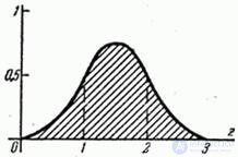
Fig. 12.6.1.

Comments
To leave a comment
Probability theory. Mathematical Statistics and Stochastic Analysis
Terms: Probability theory. Mathematical Statistics and Stochastic Analysis