5.9. Poisson law

In many problems of practice, we have to deal with random variables distributed according to a peculiar law, which is called the Poisson law.

Consider a discontinuous random variable which can only accept integer, non-negative values:

,

and the sequence of these values ​​is theoretically unlimited.

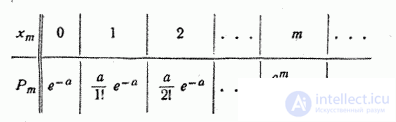
It is said that a random variable distributed according to the Poisson law, if the probability that it will take a certain value expressed by the formula

, (5.9.1)

where a is some positive quantity, called the Poisson law parameter.

Random distribution series distributed according to the Poisson law, has the form:

We first verify that the sequence of probabilities defined by formula (5.9.1) can be a series of distribution, i.e. what is the sum of all probabilities equals one. We have:

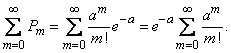
But

,

from where

.

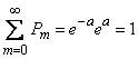In fig. Figure 5.9.1. Shows polygons of a random variable. distributed according to the Poisson law, corresponding to different values ​​of the parameter . Table 8 of the appendix shows the values for various .

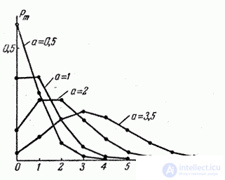
Fig. 5.9.1.

We define the main characteristics - the expectation and variance - random variable distributed according to the Poisson law. By the definition of expectation

.

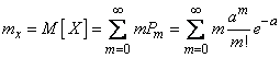The first member of the amount (corresponding to ) is equal to zero, therefore, the summation can begin with :

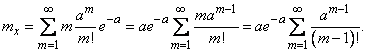
Denote ; then

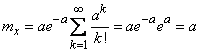. (5.9.2)

Thus, the parameter is nothing more than the expectation of a random variable .

To determine the variance, we first find the second initial moment of magnitude :

According to previously proven

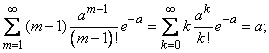
Besides,

Consequently,

Next, we find the variance of :

(5.9.3)

Thus, the variance of a random variable distributed according to Poisson’s law is equal to its expectation .

This property of the Poisson distribution is often used in practice to decide whether the hypothesis that the random variable distributed according to the Poisson law. To do this, determine from the experience of statistical characteristics - the expectation and variance - a random variable. If their values ​​are close, then this may serve as an argument in favor of the Poisson distribution hypothesis; a sharp difference in these characteristics, on the contrary, is against the hypothesis.

Define for a random variable distributed according to the Poisson law, the probability that it will take a value not less than the specified . Denote this probability :

.

Obvious likelihood can be calculated as the sum

However, it is much easier to determine it from the probability of the opposite event:

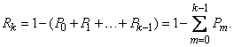(5.9.4)

In particular, the probability that the magnitude take a positive value, expressed by the formula

(5.9.5)

We have already mentioned that many practical tasks lead to the Poisson distribution. Consider one of the typical tasks of this kind.

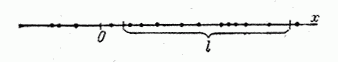
Fig. 5.9.2.

Suppose that points are randomly distributed on the abscissa axis Ox (Fig. 5.9.2). Suppose that a random distribution of points satisfies the following conditions:

1. The probability of hitting a particular number of points on the segment depends only on the length of this segment, but does not depend on its position on the abscissa axis. In other words, the points are distributed on the x-axis with the same average density. Denote this density (ie, the expectation of the number of points per unit length) .

2. The points are distributed on the x-axis independently of each other, i.e. the probability of hitting one or another number of points on a given segment does not depend on how many of them fell on any other segment that does not overlap with it.

3. The probability of hitting a small area two or more points are negligible compared to the probability of hitting a single point (this condition means the practical impossibility of two or more points coinciding).

Select on the abscissa a certain segment of length and consider a discrete random variable - the number of points falling on this segment. Possible values ​​will be

(5.9.6)

Since the points fall on the segment independently of each other, it is theoretically possible that there will be as many of them there, i.e. the series (5.9.6) is unlimited.

Prove that the random variable has a Poisson distribution law. To do this, we calculate the probability the fact that the segment will fall exactly points.

First we solve a simpler problem. Consider on the axis oh a small section and calculate the probability that at least one point falls on this area. We will argue as follows. The mathematical expectation of the number of points falling on this area is obviously equal to (since per unit length falls on average points). According to condition 3 for a small segment You can neglect the possibility of hitting him with two or more points. Therefore, the expectation the number of points falling on the plot , will be approximately equal to the probability of hitting one point on it (or, which in our conditions is equivalent, at least one).

Thus, up to infinitesimal higher order, with can be considered the probability that the plot there will be one (at least one) point equal to , and the probability that no one will be equal to .

We use this to calculate the probability hits on a segment smooth points. Divide the segment on equal parts long . We agree to call an elementary segment “Empty” if not a single point has fallen into it, and “busy” if at least one has fallen into it. According to the above, the probability that the segment will be "busy", approximately equal to ; the probability that it will be "empty" is equal to . Since, according to condition 2, the points falling into non-overlapping segments are independent, our n segments can be considered as independent “experiments”, in each of which a segment can be “occupied” with probability . Find the probability that among segments will be exactly "Busy". By the repetition theorem, this probability is

or denoting ,

(5.9.7)

When large enough this probability is approximately equal to the probability of hitting the segment smooth points, since getting two or more points per segment has a negligible probability. In order to find the exact value , it is necessary in expression (5.9.7) to go to the limit at :

(5.9.8)

Convert the expression under the limit sign:

(5.9.9)

The first fraction and the denominator of the last fraction in the expression (5.9.9) with obviously aiming for a unit. Expression from does not depend. The numerator of the last fraction can be converted as follows:

(5.9.10)

With and expression (5.9.10) tends to . Thus, it is proved that the probability of hitting exactly points per segment expressed by the formula

,

Where i.e. the value of X is distributed according to the Poisson law with the parameter .

Note that the value meaning is the average number of points per segment .

Magnitude (the probability that the magnitude of X will take a positive value) in this case expresses the probability that at least one point will fall:

. (5.9.11)

Thus, we have seen that the Poisson distribution occurs where some points (or other elements) occupy a random position independently of each other, and the number of these points that fall into some area is calculated. In our case, this “area” was a segment on the x-axis. However, our conclusion can be easily extended to the case of distribution of points on a plane (random flat field of points) and in space (random spatial field of points). It is easy to prove that if the conditions are met:

1) points are distributed in a field statistically uniform with average density ;

2) the points fall into non-overlapping regions in an independent manner;

3) dots appear singly, not in pairs, triples, etc., then the number of dots falling into any area (flat or spatial) are distributed according to the Poisson law:

,

Where - the average number of points falling into the area .

For a flat case

,

Where - area of ​​the region ; for spatial

,

Where - area volume .

Note that for the Poisson distribution of the number of points falling in a segment or region, the condition of constant density ( ) irrelevant. If two other conditions are fulfilled, then the Poisson law still holds, only the parameter and in it acquires another expression: it is obtained not by a simple density multiplication by length, area, or volume of a region, and by integrating a variable density over a segment, area, or volume. (For details on this, see n ° 19.4)

The presence of random points scattered on a line, on a plane or volume is not the only condition under which the Poisson distribution occurs. You can, for example, prove that the Poisson law is the limit for the binomial distribution:

, (5.9.12)

if simultaneously push the number of experiences to infinity and the probability - to zero, and their product keeps constant value:

. (5.9.13)

Indeed, this limiting property of the binomial distribution can be written as:

. (5.9.14)

But from the condition (5.9.13) it follows that

. (5.9.15)

Substituting (5.9.15) into (5.9.14), we obtain the equality

, (5.9.16)

which has just been proven by us on another occasion.

This limiting property of the binomial law often finds application in practice. Assume that a large number of independent experiments are made. in each of which event has a very low probability . Then to calculate the probability that event will appear exactly Once, you can use the approximate formula:

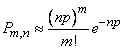, (5.9.17)

Where - the parameter of the Poisson law, which is approximately replaced by the binomial distribution.

From this property of the Poisson law — to express the binomial distribution with a large number of experiments and a low probability of an event — its name, often used in statistical textbooks: the law of rare phenomena, occurs.

Consider a few examples related to the Poisson distribution from different areas of practice.

Example 1. An average telephone density call arrives at an automatic telephone exchange. calls per hour. Considering that the number of calls in any part of the time is distributed according to the Poisson law, find the probability that in two minutes exactly three calls will arrive at the station.

Decision. The average number of calls in two minutes is:

.

According to the formula (5.9.1) the probability of receipt of exactly three calls is equal to:

Example 2. In the conditions of the previous example, find the probability that in two minutes at least one call will arrive.

Decision. By the formula (5.9.4) we have:

.

Example 3. In the same conditions, find the probability that in two minutes at least three calls will arrive.

Decision. By the formula (5.9.4) we have:

Example 4. On a loom the thread breaks on average 0.375 times during the hour of the machine. Find the probability that for a shift (8 hours) the number of thread breaks will be contained in the boundaries 2 and 4 (at least 2 and no more than 4 breaks).

Decision. Obviously

we have:

According to table 8 of the application when

Example 5. On average, a cathode is heated from a hot cathode electrons where - time elapsed since the beginning of the experience. Find the probability that over a period of time starting at the moment , exactly m electrons will fly from the cathode.

Decision. Find the average number of electrons a, departing from the cathode for a given period of time. We have:

.

According to the calculated determine the desired probability:

.

Example 6. The number of fragments that fall into a small-sized target at a given position of the break point is distributed according to the Poisson law. The average density of the fragmentation field in which the target finds itself at a given position of the break point is 3 sc / sq. The target area is equal to sq.m. To hit a target, it is enough to hit at least one fragment in it. Find the probability of hitting the target at a given position of the break point.

Decision. . By the formula (5.9.4) we find the probability of hitting at least one fragment:

.

(To calculate the value of the exponential function use table 2 of the annex).

Example 7. The average density of pathogenic microbes in one cubic meter of air is 100. A sample of 2 cubic meters is taken per sample. dm air. Find the probability that at least one microbe will be detected in it.

Decision. Taking the hypothesis of the Poisson distribution of the number of microbes in the volume, we find:

Example 8. For some goal 50 independent shots are fired. The probability of hitting the target with one shot is 0.04. Using the limit property of the binomial distribution (formula (5.9.17)), we can find the approximate probability that the target will hit: not a single projectile, one projectile, two projectiles.

Decision. We have . In table 8 of the application we find the probabilities: