Lecture
|
The model is an analogue, prototype, pattern, pattern used instead of the original for solving problems (getting answers to questions). The model is based on a limited set of known data (properties, behaviors) about the original. Building models and using models (solving problems on them) is done in order to:
Modeling is a method, the process of replacing the original with its analogue (model) with the subsequent study of the properties and behavior of the original on the model. The modeling process consists of:
The model instead of the original object is used in cases when the experiment is dangerous, expensive, takes place on an inconvenient scale of space and time (long-term, too short, long ...), impossible, unique, unattractive, etc. Let's illustrate this:
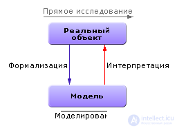
The modeling process is the process of transition from a real area to a virtual (model) through formalization, then the model is studied (modeling itself) and, finally, the results are interpreted as a reverse transition from a virtual to a real area. This path replaces the direct study of an object in a real area, that is, a frontal or intuitive solution of the problem. So, in the simplest case, the technology of modeling involves 3 stages: formalization, modeling itself, interpretation (Fig. 1.1).
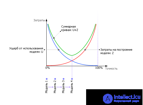
If clarification is required, these stages are repeated again and again: formalization (design), modeling, interpretation. Spiral! Up the circle. In more detail the entire development cycle is shown in Fig. 1.14, which reflects the methods, methods, techniques by which each of the stages is implemented. Since modeling is a way of replacing a real object with its analog, the question arises: how much does the analog have to correspond to the original object? Option 1: compliance - 100%. It is obvious that the accuracy of the solution in this case is maximum, and the damage from the application of the model is minimal. But the costs of building such a model are infinitely large, since the object is repeated in all its details; in fact, exactly the same object is created by copying it to atoms (which in itself does not make sense). Option 2: compliance - 0%. The model is not at all like a real object. Obviously, the accuracy of the solution is minimal, and the damage from the application of the model is maximum, infinite. But the cost of building such a model is zero. Of course, options 1 and 2 are extremes. In fact, the model is created for reasons of compromise between the costs of its construction and the damage from the inaccuracy of its application. This is a point between two infinities. That is, when modeling, it should be borne in mind that the researcher (modeler) should strive for the optimum of the total costs, including the damage from the application and the cost of making the model (see Fig. 1.2).
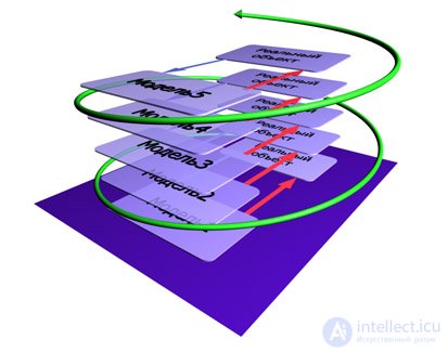
Sum up the two cost curves - you get one total cost curve. Find the optimum on the total curve: it lies between these extreme variants. It can be seen that inaccurate models are not needed, but absolute accuracy is also not needed, and it is impossible. Frequent and common misconception when building models is to demand "as accurately as possible." “The model is the search for the finite in the infinite” - this thought belongs to DI Mendeleev. What is dropped to transform the infinite into the finite? Only essential aspects representing the object are included in the model, and all others are discarded (infinite majority). The essential or non-essential aspect of the description is determined according to the purpose of the study. That is, each model is made up for some purpose. When starting a simulation, the researcher must determine the goal, separating it from all possible other targets, the number of which is apparently infinite. Unfortunately, indicated in fig. 1.2 the curve is speculative and really cannot be built before the start of the simulation. Therefore, in practice, they act in this way: they move along the accuracy scale from left to right, that is, from simple models ("Model 1", "Model 2" ...) to more and more complex ("Model 3", "Model 4" ...). And the modeling process has a cyclical spiraling character: if the constructed model does not meet the accuracy requirements, then it is detailed, refined in the next cycle (see Fig. 1.3).
Improving the model, make sure that the effect of the complexity of the model exceeds the associated costs. As soon as the researcher notices that the cost of refining the model exceeds the effect of accuracy when applying the model, we should stop, since the optimum point has been reached. This approach always guarantees the return on investment. From all this it follows that there may be several models: approximate, more accurate, more precise, and so on. Models form a series. Moving from option to option, the researcher improves the model. To build and improve models, they need continuity, version tracking tools, and so on, that is, modeling requires a tool and relies on technology. |
|
|
Sometimes models are written in programming languages, but this is a long and expensive process. Mathematical packages can be used for modeling, but experience shows that they usually lack many engineering tools. The best is to use a simulation environment. In our course, the Stratum-2000 Design and Modeling System was chosen as such an environment. Laboratory work and demonstrations that you will find in the course should be launched as projects of the Stratum-2000 environment. A model made with regard to the possibility of its modernization, of course, has drawbacks, for example, a low code execution speed. But there are undeniable merits. The structure of the model, connections, elements, subsystems is visible and saved. You can always go back and redo something. The mark in the model design history has been preserved (but when the model is debugged, it makes sense to remove official information from the project). In the end, the model, which surrenders to the customer, can be framed in the form of a specialized workstation (ARM), written in a programming language, attention in which is mainly paid to the interface, speed parameters and other consumer properties that are important for customer AWP is certainly an expensive thing, so it is released only when the customer has fully tested the project in the modeling environment, made all the comments and is committed to no longer changing his requirements. Modeling is an engineering science, problem solving technology. This remark is very important. Since technology is a way to achieve results with a well-known quality and guaranteed costs and terms, modeling, as a discipline:
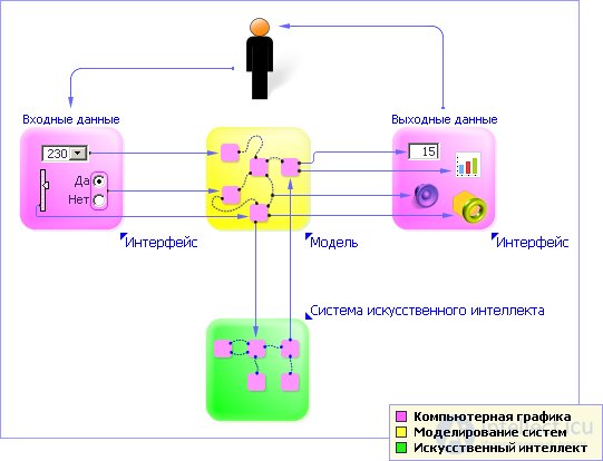
Related modeling subjects are: programming, mathematics, operations research. Programming - because often the model is implemented on an artificial carrier (plasticine, water, bricks, mathematical expressions ...), and the computer is one of the most universal information carriers and is also active (imitates plasticine, water, bricks, counts mathematical expressions, etc.) ). Programming is a way of presenting the algorithm in language form. Algorithm is one of the ways to represent (reflect) a thought, process, or phenomenon in an artificial computing environment, which is a computer (von Neumann architecture). The specificity of the algorithm is to reflect the sequence of actions. Simulation can use programming if the object being modeled is easy to describe in terms of its behavior. If it is easier to describe the properties of an object, then programming is difficult to use. If the modeling environment is not built on the basis of the von Neumann architecture, programming is almost useless. What is the difference between algorithm and model? An algorithm is a process of solving a problem by implementing a sequence of steps, while a model is a set of potential properties of an object. If you put a question to the model and add additional conditions in the form of initial data (connection with other objects, initial conditions, restrictions), then the researcher can solve it with respect to unknowns. The process of solving a problem can be represented by an algorithm (but other solutions are also known). In general, examples of algorithms in nature are unknown; they are the product of the human brain, a mind capable of establishing a plan. Actually, the algorithm is the plan developed in a sequence of actions. It is necessary to distinguish between the behavior of objects associated with natural causes, and the craft of the mind, controlling the course of motion, predicting the result based on knowledge and choosing an expedient variant of behavior. So: model + question + additional conditions = task. Mathematics is a science that provides the possibility of calculating models reducible to the standard (canonical) form. The science of finding solutions of analytical models (analysis) by means of formal transformations. Operations research is a discipline that implements ways to research models in terms of finding the best control actions on a model (synthesis). For the most part deals with analytical models. Helps to make decisions using built models. Design is the process of creating an object and its model; modeling - a way to assess the result of the design; modeling without design does not exist. Electrical engineering, economics, biology, geography and others can be recognized as related disciplines for modeling in the sense that they use modeling methods to study their own applied object (for example, landscape model, electric circuit model, cash flow model, etc.). Nearby are the disciplines "Computer graphics" and "Models and methods of artificial intelligence" (see. Fig. 1.4).
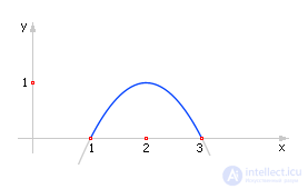
Computer graphics helps to organize a convenient natural interface to manage the model, to monitor its reactions. It is important to understand that the user interacts with the model indirectly, namely through the interface: on the one hand, he sends her source (input) data (for example, using input windows, buttons, engines, command line, etc.), on the other - looks at the result of the model, that is, it receives output data via the interface. Artificial intelligence implies the construction of higher models (for example, adaptive ones that know how to self-tune, know how to create each other, etc.). It is understood that the model of intelligence in itself is able to build models of applied objects and systems; an explanation of how this is done is given in the course “Models and Methods of Artificial Intelligence”. At the same time, we note that a number of researchers, speaking of artificial intelligence, are referring to the use of models (learning, reproduction, language, etc.) for studying and imitating one of the most complex systems in the Universe - man. Note that artificial intelligence is a fairly large model that contains extensive information about the world and meta-models that can complete it. Meta-models have a great similarity with the person imitated by them. Depending on the carrier, there are models: natural, mental, mathematical, imitation, graphic, photographic, and so on. Each of the models has a different ability to predict the properties of the object. For example, from a photograph of a person in full face one can hardly truly imagine what his nape looks like. An approximation in the form of a three-dimensional model is much better, but can it be determined with its help when, for example, a 50-cm-long hair grows in a virtual person? The simulation model is even more informative. But the most valuable are models suitable for solving problems, that is, possessing predictive properties and able to answer questions. It is necessary to distinguish two concepts - “model” and “task”. The model connects variables with each other by laws. These laws are valid regardless of what the challenge is now facing us. The model is objective, it is similar to the world that surrounds us, and contains information about it. The structure of the world (in a general sense) is immutable, fundamental, the model, therefore, too. And a person, as a subjective being, having its own goals, often changing desires, sets, depending on his needs, new tasks every time, he demands to solve the problems arising from him. He poses questions for the world around him, whose laws cannot be ignored. It is convenient to pose questions to a model that contains the necessary information about the world.Therefore, the task is a set of issues and models. It is possible to ask the model all new and new questions and not to change the model, but to change the task. That is, a model is a way of finding answers to questions. To answer the question posed, the model must be transformed according to the rules ensuring its equivalence, to the form corresponding to the answer to the question. This means that the model must be formed according to the rules of a certain algebra (algebra is a transformation rule). A procedure that helps to apply such rules to a model is called a method. Consider an example. Модель падения тела под углом к горизонту содержит информацию о координатах траектории, заданных в осях ( x , y ): y = – x 2 + 4 · x – 3 (координаты тела в полете) — см. рис. 1.5.
Модель связывает две переменные y и x законом f ( y , x ) = 0. Модель может быть расширена некоторыми исходными данными, например, так: y = – x 2 + 4 · x – 3, y = 0 (интересуют не все возможные значения y , а только точки на поверхности Земли). y = 0 — это тоже закон, но более мелкого масштаба. Такие уравнения могут появляться и исчезать в зависимости от исследуемой проблемы. Обычно их называют гипотезами. Вопрос: x = ? Теперь модель и вопрос вместе образовали задачу:
Трактовать задачу можно так: при каких значениях x тело окажется на поверхности Земли? Модель подразумевает, что исследователь может решать с её помощью прямые и обратные задачи. Прямая задача не требует алгебраических преобразований, достаточно только арифметических подстановок: x = 2, y = – x 2 + 4 · x – 3, y = ?. Ответ: y = 1. То есть, если на вход модели подать значение 2, то на выходе модели будет значение 1 — см. рис. 1.6.
Обратная задача: y = 0, y = – x 2 + 4 · x – 3, x = ? Ответ: x = 1, x = 3. То есть ответ говорит: чтобы на выходе модели обеспечить значение 0, надо, чтобы на вход модели было подано значение 1 (или 3). И в первом, и во втором случае мы в разной мере преобразовывали модель, но всегда так, чтобы на входе у неё была известная величина, а на выходе — неизвестная. В первом варианте y := – x 2 + 4 · x – 3. Во втором варианте модель преобразуется к виду: 0 = – x 2 + 4 · x – 3. Здесь мы опустили ряд преобразований, известных из курса средней школы, а именно:
Преобразования происходили с учётом правил алгебры. Если бы правила алгебры были нам неизвестны, то решить обратную задачу нам бы не удалось. А значит, не удалось бы ответить на поставленный вопрос: « x = ?». Способность модели преобразовываться с помощью алгебры даёт возможность в дальнейшем использовать её многократно для решения различных задач, делать на ней прогнозы. Сравните: телефонный справочник — это тоже своеобразная модель, но какие прогнозы вы можете сделать, какие обратные задачи решить? Как вычислить фамилию абонента по номеру телефона? Какую алгебру вы используете? Поэтому, создавая модель, следует обязательно думать о том, какой алгеброй она будет преобразовываться. Создавать алгебру следует параллельно с моделью или использовать уже готовую алгебру и не отходить при построении модели от её правил. Ещё один тип задач, который приходится решать на моделях — задачи настройки модели. Let's give an example.For what values of the parameter a will the model y = a · x 2 + 4 · x - 3 provide y = 9 with x = 2? Solve the system of equations:
or
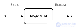
Further, according to the rules of arithmetic and algebra, we get the answer: a = 1. From the shown in fig. 1.7 structural image of the model, you can go to another, mathematical, her mind: Y = M ( X ).
Model - a pattern that converts input values to the weekend. And as is known from mathematics, with the expression Y = M ( X ), three types of problems can be solved, which are listed in Table. 1.1.
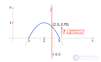
Ряд моделей может быть недоопределён — это означает, что вариантов ответов много (два, три, сто или бесконечное множество). Если нужен один ответ, то проблему надо доопределять, дополнять условиями. «Недоопределён» означает, что можно произвольно, кроме гипотез, законов, ответа, потребовать дополнительно выполнение ещё каких-то условий. Возможно, при построении модели что-то не было учтено, не хватает каких-то законов. Рецепт понятен: модель надо достроить. Но может быть и по-другому. Решений много и есть, видимо, лучшие решения, и есть похуже. Тогда для нахождения лучшего решения следует сузить область решений, накладывая определённые ограничения, чтобы отсеять остальные. Такие задачи часто называют задачами управления. Часть определений, которым надо безусловно удовлетворить, называются ограничениями. Часть определений, относительно которых высказывают только пожелания («быть как можно больше или меньше»), называются критериями. В целом получается обратная задача. А то, что надо определить — управляемая переменная. То есть интересуются: как следует изменить входной параметр (управление), чтобы обеспечить выполнение законов, не выйти за ограничения и чтобы при этом критерий принял наилучшее значение? Example. Модель: y = – x 2 + 4 · x – 3. Вопрос: x = ? Доопределение модели: y должен быть максимизирован, x ≥ 2.5. Так как y должен быть максимизирован, то мы должны стараться двигаться вверх вдоль графика функции (рис. 1.8) и следить, чтобы значение x не стало меньше 2.5. Как видно из рисунка, значение y станет максимальным при x = 2.5. Ответ: y = 0.75, x = 2.5.
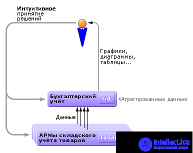
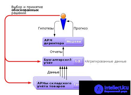
Отметим, что создать модель бывает проще, чем сразу дать себе ответ на интересующий вопрос. Наверное, на практике вы замечали, что часто гораздо проще составить уравнения, чем угадать решение задачи. Например: решено разделить огромный шар размером с Землю на две половинки, полученную половинку снова поделить пополам и так далее. Попробуйте ответить на вопрос: сколько раз ( n ) надо провести такую операцию, чтобы размер делимой частички в результате достиг размера атома? Наверняка, сразу ответить на этот вопрос не удастся, интуиция подводит, придётся составить модель. Пусть D = 6 400 км = 6 400 000 м — диаметр шара (Земли), а d = 10 –9 м — диаметр атома. Тогда модель есть выражение: 2 n = D / d или 2 n = 6 400 000/10 –9 . Отсюда получаем: 2 n = 6.4 · 10 15 или n = log 2 (6.4 · 10 15 ). Итак, приближённо, n = 53. Неожиданный результат, не правда ли?! Можно ли было его предугадать? Ещё несколько примеров. Тривиальные модели: x = 5°; телефон друга Сидорова — 912–36–54. Такие модели не несут в себе прогностических свойств, поскольку на основе известной информации невозможно вычислить каким-либо образом другую информацию. Зная телефон одного друга Сидорова, невозможно вычислить телефон другого его друга. Это так называемые пра-модели (pra-model). Фактически это данные. Заметим, что недооценка в современных условиях понятия моделирования ведёт к использованию в АРМах коммерческого назначения только данных. Именно поэтому такие АРМы не способны решать прогностические задачи и решают, в основном, только учётные задачи (см. рис. 1.9).
Чтобы проиграть ситуацию на предприятии на будущее, узнать, к чему приведёт то или иное решение, следует в состав АРМов включать модели (см. рис. 1.10).
In fig. 1.11 показана пирамида моделей, различных по степени прогностичности.
Please note: the “Model” level is “fed” with information structured by the type of the previous “P-Model” level, that is, it consumes data at the input, processes it and returns data too, that is, lower-level models (prag-models). We emphasize once again that the data - this is also a model! The “Supra-model” level consumes the model input as objects and operations, processes them and returns models (an example of such supra-models can be grammars that can transform models (equations). See Fig. 1.12 for more details). This principle is valid for all subsequent (higher) levels. The pyramid in fig. 1.11 is represented in the form of functional levels; This means that each subsequent level is more powerful than the previous one, that is, it allows you to get a larger, more powerful, high-quality result. Models can take various forms, depending on the way of thinking of the researcher, his view of the world, the algebra used. The use of various mathematical tools subsequently leads to different possibilities in solving problems. Models can be:
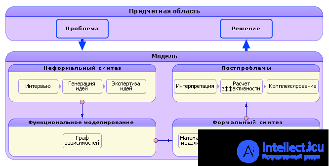
Phenomenological models are strongly tied to a specific phenomenon. Changing the situation often leads to the fact that it is quite difficult to use the model in new conditions. This is due to the fact that during the compilation of the model it was not possible to construct it from the point of view of similarity to the internal structure of the system being modeled. The phenomenological model conveys external similarity. An abstract model reproduces the system from the point of view of its internal structure, copies it more accurately. It has more features, a wider class of tasks. Active models interact with the user; they can not only, as passive, give answers to the user's questions when he asks for it, but also activate the dialogue themselves, change its line, have their own goals. All this happens due to the fact that active models can change themselves. Static models describe phenomena without development. Dynamic models trace the behavior of systems, so they use in their writing, for example, differential equations derived from time. Discrete and continuous models. Discrete models change the state of variables abruptly, because they do not have a detailed description of the relationship between causes and effects, part of the process is hidden from the researcher. Continuous models are more accurate, contain information about the details of the transition. Deterministic and stochastic models. If the effect is precisely determined by the cause, then the model represents the process is determined. If, due to the lack of knowledge of the details, it is not possible to describe the exact relationship between causes and effects, and perhaps only the description as a whole, statistically (which often happens for complex systems), then the model is constructed using the notion of probability. Distributed, structural, concentrated models. If a parameter describing a property of an object has the same value at any of its points (although it may vary in time!), Then this is a system with lumped parameters. If the parameter takes different values at different points of the object, then they say that it is distributed, and the model describing the object is distributed. Sometimes the model copies the structure of the object, but the parameters of the object are concentrated, then the model is structural. Functional and object models. If the description is from the point of view of behavior, then the model is built on a functional basis. If the description of each object is separated from the description of another object, if the properties of the object are described, from which its behavior follows, then the model is object-oriented. Each approach has its advantages and disadvantages. Different mathematical devices have different capabilities (power) for solving problems, different needs for computing resources. The same object can be described in various ways. The engineer must correctly apply this or that idea, based on current conditions and the problem before him. The above classification is ideal. Models of complex systems usually have a complex form, use several representations in their structure at once. If it is possible to reduce the model to one type for which algebra has already been formulated, then the study of the model, the solution of problems on it is greatly simplified, it becomes typical. For this, the model should be in various ways (simplification, re-designation and others) reduced to a canonical form, that is, to a form for which algebra has already been formulated, its methods. Depending on the type of model used (algebraic, differential, graphs, etc.), different mathematical tools are used at different stages of its research. The full (extended) version of the scheme shown in Fig. 1.13, see fig. 1.14. After reading the entire course of lectures, it is recommended to return to fig. 1.14 and in more detail, at a deeper level, familiarize yourself with it.
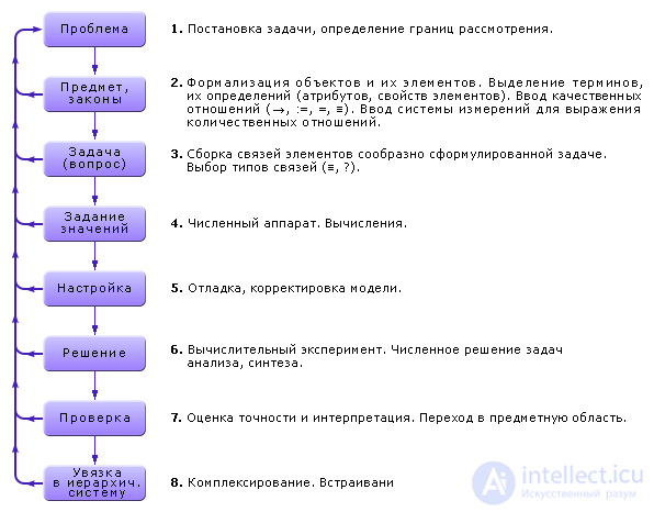
In fig. 1.15 presents the stages of building a model.
The spiral, which was considered in Fig. 1.3, is presented in fig. 1.15 as a round. But pay attention to the possibility of returning from each stage to an earlier (or earlier) when an error is detected. The spiral has a rather complicated look, stitched with additional links. A general description of the simulation technology is located in the help file of the Stratum-2000 system in the “Modeling Theory” section (“Help” > “Modeling Theory”). First, this section should be read fluently, and then in detail - after you have mastered the entire course and have gained experience in describing objects using examples and experience gained during the course work. Of course, modeling, as already mentioned, in conjunction with the design is a technology for solving problems and problems. But each technology still has a border beyond which it is less effective. Such a boundary exists here. Look again at pic. 1.13. It is obvious that the first stages solve less formalized tasks, and the subsequent ones - more and more formal ones. Accordingly, the methods of the first stages are less formalized, and the subsequent ones are more formal, powerful. This means that the most difficult and crucial stages for the modeler are the first. Here, more intuitive solutions are required of him. And the error at earlier stages affects further decisions, it is necessary to come back and redo much more than at the last stages. Therefore, successful solutions at the first stages cause keen interest of system engineers, the science of modeling shows increased attention to them. Since formal methods are easily automated, the last stages of the scheme are supported by software products and are easily accessible to end users, but the most interesting today are software products that support the first stages - systems that help formalize tasks. As well as systems that provide end-to-end design, brought to the modeling and final implementation (automatic generation of code according to the project description). Two directions can be mentioned here. The first is instrumental. The designer needs a tool for the formal description of the object under consideration. Several such tools are known: RationalRose, Analytic, IDEF using SADT technology, Stratum. There are tools that suggest solutions, there are just passive sets, libraries. One of the tools for finding solutions is the technology of ALRIZ; following its algorithm, answering questions of this technology, it is possible to come to a decision with guarantee. The second way is analytical systems that derive from the facts of knowledge. We will talk about them in our next course - “Models and Methods of Artificial Intelligence”. As an example, let's see how to detect and then describe the pattern. Suppose that we need to solve the “Cuts problem”, that is, we need to predict how many cuts will be required in the form of straight lines to divide the figure (fig. 1.16) into a given number of pieces (for example, it is enough that the figure is convex). Let's try to solve this problem manually.
From fig. 1.16 it can be seen that with 0 cuts 1 piece is formed, with 1 cut 2 pieces are formed, with two - 4, with three - 7, with four - 11. Can you say in advance how many cuts are needed to form, for example, 821 pieces ? In my opinion, no! Why do you find it difficult? - You do not know the pattern K = f ( P ), where K is the number of pieces, P is the number of cuts. How to detect patterns? Let's make the table connecting known to us numbers of pieces and cuts.
While the pattern is not clear. Therefore, we consider the differences between individual experiments, see how the result of one experiment differs from another. Having understood the difference, we will find a way to go from one result to another, that is, a law connecting K and P.
Already some pattern manifested, is not it? Calculate the second difference.
It is obvious that further to continue the procedure for calculating differences makes no sense. Now everything is simple. The function f is called the generating function. If it is linear, then the first differences are equal to each other. If it is quadratic, then the second differences are equal to each other. And so on. The function f is a special case of Newton's formula:
The coefficients a , b , c , d , e for our quadratic function f are in the first cells of the rows of the experimental table 1.5.
So, there is a pattern, and it is as follows: K = a + b · p + c · p · ( p - 1) / 2 = 1 + p + p · ( p - 1) / 2 = 0.5 · p 2 + 0.5 · p + | |||||||||||||||||||||||||||||||||||||||||||||||||||||||||||||||||||||||||||||||||||||||||||||||||||||||||||||||||||||||||||||||||||||||||||||||||||||||||||||||||||||||||||||||||||||||||||||||||||||||||||||||||||||||||||||||||||||||||||||||||||||||||||||||||||||||||||||||||||||||||||||||
продолжение следует...
Часть 1 The concept of modeling. Ways to present models
Часть 2 Analytical way of presenting task 1 - The concept of


Comments
To leave a comment
System modeling
Terms: System modeling