Random Number Generators

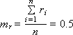
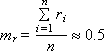
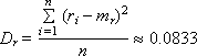
The Monte Carlo method (see Lecture 21. Statistical modeling) is based on the generation of random numbers that should be evenly distributed in the interval (0; 1).

If the generator produces numbers that are offset in some part of the interval (some numbers fall out more often than others), then the result of solving the problem solved by the statistical method may turn out to be incorrect. Therefore, the problem of using a good generator of truly random and really evenly distributed numbers is very serious.

The expectation m _r and the variance D _{r of} such a sequence consisting of n random numbers r _i should be as follows (if these are really uniformly distributed random numbers in the range from 0 to 1):

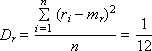
If the user needs the random number x to be in the interval ( a ; b ), other than (0; 1), use the formula x = a + ( b - a ) · r , where r is a random number from the interval (0; one). The legality of this transformation is demonstrated in fig. 22.1.

Fig. 22.1. The scheme of converting a number from the interval (0; 1) to the interval (a; b)

Now x is a random number evenly distributed in the range from a to b .

Fig. 22.2. Frequency pattern of random numbers generated by a real generator

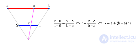
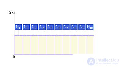
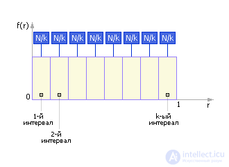
Note that, ideally, the density distribution curve of random numbers would look like that shown in Fig. 22.3. That is, in the ideal case, the same number of points falls into each interval: N _i = N / k , where N is the total number of points, k is the number of intervals, i = 1, ..., k .

Fig. 22.3. Frequency pattern of random numbers theoretically generated by the ideal generator

It should be remembered that the generation of an arbitrary random number consists of two stages:

• generation of a normalized random number (that is, uniformly distributed from 0 to 1);
• conversion of normalized random numbers r _i to random numbers x _i , which are distributed according to the user’s (arbitrary) distribution law or in the required interval.

Random number generators by the method of obtaining numbers are divided into:

• physical;
• tabular;
• algorithmic.

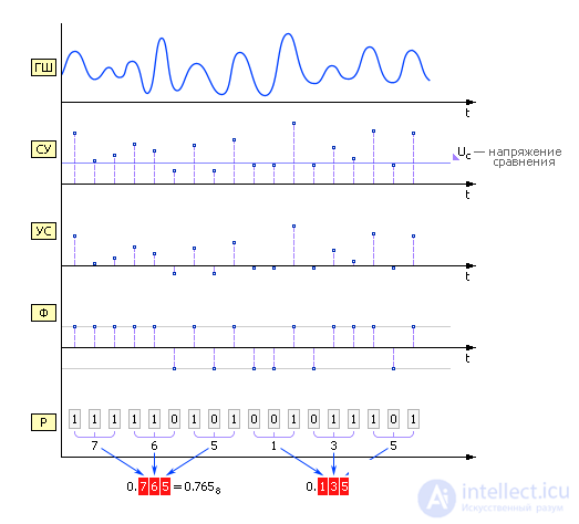
Physical RNG

An example of physical RNGs can be: a coin ("eagle" - 1, "tails" - 0); dice; divided into sectors with numbers drum with an arrow; instrumental noise generator (GSH), which is used as a noisy thermal device, for example, a transistor (Fig. 22.4–22.5).

Fig. 22.4. The scheme of the hardware method of generating random numbers

Fig. 22.5. Chart of obtaining random numbers by the hardware method

Tabular RNG

Table RNGs use specially compiled tables containing verified uncorrelated, that is, completely independent from each other, figures as a source of random numbers. In tab. 22.1 the small fragment of such table is resulted. By going around the table from left to right from top to bottom, you can get random numbers evenly distributed from 0 to 1 with the required number of decimal places (in our example, we use three signs for each number). Since the numbers in the table are independent of each other, the table can be bypassed in different ways, for example, from top to bottom, or from right to left, or, say, you can select numbers that are in even positions.

The advantage of this method is that it gives really random numbers, since the table contains verified uncorrelated numbers. Disadvantages of the method: it takes a lot of memory to store a large number of digits; the great difficulties of generating and checking such tables, repeats when using the table no longer guarantee the randomness of the numerical sequence, and hence the reliability of the result.

Here is a table containing 500 absolutely random tested numbers (taken from the book by I. G. Venetsky, V. I. Venetskaya "Basic mathematical-statistical concepts and formulas in economic analysis").

Algorithmic RNG

The numbers generated by these RNGs are always pseudo-random (or quasi-random), that is, each subsequent generated number depends on the previous one:

r _{i + 1} = f ( r _i ).

Sequences made up of such numbers form loops, that is, there is a loop that repeats infinitely many times. Repeating cycles are called periods.

The strength of the RNG data is speed; generators practically do not require memory resources, are compact. Disadvantages: numbers cannot be fully called random, since there is a dependency between them, as well as the presence of periods in a sequence of quasi-random numbers.

Consider several algorithmic methods for obtaining RNG:

• mid squares method;
• method of middle works;
• mixing method;
• linear congruential method.

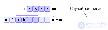
Square method

There is some four-digit number R 0. This number is squared and entered in R 1. Then, from R 1, the middle is taken (four middle digits) - the new random number - and written in R 0. Then the procedure is repeated (see Fig. 22.6) . Note that in fact, as a random number, it is necessary not to take ghij , but 0.ghij — with a zero assigned and a decimal point assigned to the left. This fact is shown in fig. 22.6, and in subsequent similar figures.

Fig. 22.6. Diagram of the method of mean squares

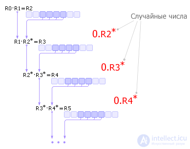
Disadvantages of the method: 1) if at some iteration the number R 0 becomes zero, then the generator degenerates, therefore the correct choice of the initial value R 0 is important; 2) the generator will repeat the sequence in M ⁿ steps (at best), where n is the width of the number R 0, M is the base of the number system.

For an example in fig. 22.6: if the number R 0 is represented in binary number system, then the sequence of pseudo-random numbers will repeat in 2 ⁴ = 16 steps. Note that the repetition of the sequence can occur earlier if the initial number is chosen unsuccessfully.

The method described above was proposed by John von Neumann and dates back to 1946. Since this method was unreliable, it was quickly abandoned.

Method of the middle works

The number R 0 is multiplied by R 1, the midpoint R 2 ^* is extracted from the result R 2 (this is the next random number) and multiplied by R 1. This scheme calculates all subsequent random numbers (see Fig. 22.7).

Fig. 22.7. Diagram of the method of medial works

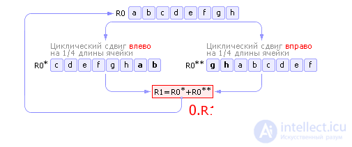
Mixing method

The shuffle method uses round-robin cell contents to the left and right. The idea of ​​the method is as follows. Let the initial number R 0 be stored in the cell. Cyclically shifting the contents of the cell to the left by 1/4 of the cell length, we obtain the new number R 0 ^* . Similarly, cyclically shifting the contents of the cell R 0 to the right by 1/4 of the cell length, we get the second number R 0 ^** . The sum of the numbers R 0 ^* and R 0 ^** gives a new random number R 1. Then R 1 is entered into R 0, and the entire sequence of operations is repeated (see Fig. 22.8).

Fig. 22.8. Mixing scheme

Note that the number obtained by summing up R 0 ^* and R 0 ^** may not fit completely in cell R 1. In this case, the extra digits should be discarded from the resulting number. We explain this for rice. 22.8, where all cells are represented by eight binary digits. Let R 0 ^* = 10010001 ₂ = 145 ₁₀ , R 0 ^** = 10100001 ₂ = 161 ₁₀ , then R 0 ^* + R 0 ^** = 100110010 ₂ = 306 ₁₀ . As you can see, the number 306 occupies 9 digits (in binary number system), and the cell R 1 (like R 0) can hold a maximum of 8 digits. Therefore, before entering a value in R 1, it is necessary to remove one “extra”, the leftmost bit from among 306, with the result that 00110010 ₂ = 50 _{10 is} already going to R 1. Also note that in languages ​​such as Pascal, the “cutting off” of extra bits when a cell overflows is performed automatically in accordance with a given type of variable.

Linear congruential method

The linear congruential method is one of the simplest and most commonly used at the present time procedures that imitate random numbers. This method uses mod ( x , y ) operation, which returns the remainder of the division of the first argument by the second. Each subsequent random number is calculated based on the previous random number using the following formula:

r _{i + 1} = mod ( k · r _i + b , M ).

The sequence of random numbers obtained using this formula is called a linear congruent sequence. Many authors call the linear congruent sequence with b = 0 the multiplicative congruential method, and with b ≠ 0 - the mixed congruent method.

For a high-quality generator, you need to select the appropriate factors. It is necessary that the number M be quite large, since the period can not have more M elements. On the other hand, the division used in this method is a rather slow operation, so for a binary computing machine it will be logical to choose M = 2 ^N , since in this case finding the remainder of the division is reduced inside the computer to a binary logical operation “AND”. The choice of the largest prime number M , which is less than 2 ^{N, is} also widespread: in the special literature, it is proved that in this case the lower digits of the random number r _{i + 1} obtained behave as randomly as the older ones, which has a positive effect on the entire sequence of random numbers in general. As an example, one of the Mersenne numbers is equal to 2 ³¹ - 1, and thus, M = 2 ³¹ - 1.

One of the requirements for linear congruent sequences is as long a period as possible. The length of the period depends on the values ​​of M , k and b . The theorem we give below allows us to determine whether it is possible to achieve a period of maximum length for specific values ​​of M , k, and b .

Theorem . A linear congruent sequence defined by the numbers M , k , b and r ₀ has a period of length M if and only if:

• the numbers b and M are coprime;
• k - 1 multiple of p for each prime p that is a divisor of M ;
• k - 1 is a multiple of 4, if M is a multiple of 4.

Finally, in conclusion, we consider a couple of examples of using the linear congruential method for generating random numbers.

It was found that a series of pseudo-random numbers generated from the data from Example 1 would be repeated every M / 4 numbers. The number q is set arbitrarily before the start of the calculations, however, it should be borne in mind that the series seems to be random for large k (and hence q ). The result can be slightly improved if b is odd and k = 1 + 4 · q - in this case, the series will be repeated every M numbers. After a long search for k, the researchers settled on the values ​​of 69069 and 71365.

A random number generator using the data from Example 2 will produce random, non-repeating numbers with a period of 7 million.

A multiplicative method for generating pseudo-random numbers was proposed by D. G. Lehmer in 1949.

Check the quality of the generator

The quality of the entire system and the accuracy of the results depend on the quality of the RNG. Therefore, the random sequence generated by the RNG must satisfy a variety of criteria.

Carried out checks are of two types:

• checks for uniform distribution;
• checks on statistical independence.

Checks for uniform distribution

1) RNG should give close to the following values ​​of statistical parameters characteristic of a uniform random law:

- expected value; - dispersion; - standard deviation.

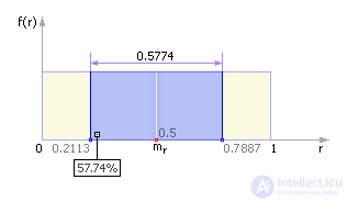
2) Frequency test

The frequency test allows you to find out how many numbers fall into the interval ( m _r - σ _r ; m _r + σ _r ), that is (0.5 - 0.2887; 0.5 + 0.2887) or, ultimately, (0.2113; 0.7887). Since 0.7887 - 0.2113 = 0.5774, we conclude that in a good RNG about 57.7% of all random numbers dropped out should fall into this interval (see. Fig. 22.9).

Fig. 22.9. Frequency chart ideal RNG in case of checking it for a frequency test

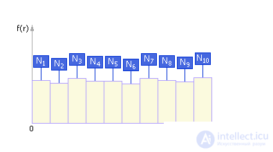
It is also necessary to take into account that the number of numbers falling within the interval (0; 0.5) should be approximately equal to the number of numbers falling within the interval (0.5; 1).

3) Check by criterion "chi-square"

The chi-square test (χ ² test) is one of the most well-known statistical criteria; It is the main method used in combination with other criteria. The chi-square test was proposed in 1900 by Karl Pearson. His remarkable work is regarded as the foundation of modern mathematical statistics.

For our case, the chi-square test will allow us to find out how close the real RNG created by us is close to the RNG standard, that is, whether it satisfies the requirement of uniform distribution or not.

The frequency diagram of the reference RNG is shown in Fig. 22.10. Since the distribution law of the reference RNG is uniform, the (theoretical) probability p _i of numbers falling into the i -th interval (all of these intervals k ) is equal to p _i = 1 / k . And, thus, exactly k p · N numbers fall into each of the k intervals ( N is the total number of generated numbers).

Fig. 22.10. Frequency chart reference RNG

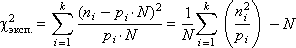
A real RNG will produce numbers distributed (moreover, not necessarily uniformly!) Over k intervals and will fall into each interval by n _i numbers (in the sum n ₁ + n ₂ + ... + n _k = N ). How do we determine how well tested RNG is good and close to the reference? It is quite logical to consider the squares of differences between the obtained number of numbers n _i and the “reference” p _i · N. Add them up, and as a result we get:

χ ² _exp. = ( n ₁ - p ₁ · N ) ² + ( n ₂ - p ₂ · N ) ² +… + ( n _k - p _k · N ) ² .

Из этой формулы следует, что чем меньше разность в каждом из слагаемых (а значит, и чем меньше значение χ ² _эксп. ), тем сильнее закон распределения случайных чисел, генерируемых реальным ГСЧ, тяготеет к равномерному.

В предыдущем выражении каждому из слагаемых приписывается одинаковый вес (равный 1), что на самом деле может не соответствовать действительности; поэтому для статистики «хи-квадрат» необходимо провести нормировку каждого i -го слагаемого, поделив его на p _i · N :

Наконец, запишем полученное выражение более компактно и упростим его:

Мы получили значение критерия «хи-квадрат» для экспериментальных данных.

In tab. 22.2 приведены теоретические значения «хи-квадрат» (χ ² _теор. ), где ν = N – 1 — это число степеней свободы, p — это доверительная вероятность, задаваемая пользователем, который указывает, насколько ГСЧ должен удовлетворять требованиям равномерного распределения, или p — это вероятность того, что экспериментальное значение χ ² _эксп. будет меньше табулированного (теоретического) χ ² _теор. или равно ему .

Приемлемым считают p от 10% до 90% .

Если χ ² _эксп. много больше χ ² _теор. (то есть p — велико), то генератор не удовлетворяет требованию равномерного распределения, так как наблюдаемые значения n _i слишком далеко уходят от теоретических p _i · N и не могут рассматриваться как случайные. Другими словами, устанавливается такой большой доверительный интервал, что ограничения на числа становятся очень нежесткими, требования к числам — слабыми. При этом будет наблюдаться очень большая абсолютная погрешность.

Еще Д. Кнут в своей книге «Искусство программирования» заметил, что иметь χ ² _эксп. маленьким тоже, в общем-то, нехорошо, хотя это и кажется, на первый взгляд, замечательно с точки зрения равномерности. Действительно, возьмите ряд чисел 0.1, 0.2, 0.3, 0.4, 0.5, 0.6, 0.7, 0.8, 0.9, 0.1, 0.2, 0.3, 0.4, 0.5, 0.6, … — они идеальны с точки зрения равномерности, и χ ² _эксп. будет практически нулевым, но вряд ли вы их признаете случайными.

Если χ ² _эксп. много меньше χ ² _теор. (то есть p — мало), то генератор не удовлетворяет требованию случайного равномерного распределения, так как наблюдаемые значения n _i слишком близки к теоретическим p _i · N и не могут рассматриваться как случайные.

А вот если χ ² _эксп. лежит в некотором диапазоне, между двумя значениями χ ² _теор. , которые соответствуют, например, p = 25% и p = 50%, то можно считать, что значения случайных чисел, порождаемые датчиком, вполне являются случайными.

При этом дополнительно надо иметь в виду, что все значения p _i · N должны быть достаточно большими, например больше 5 (выяснено эмпирическим путем). Только тогда (при достаточно большой статистической выборке) условия проведения эксперимента можно считать удовлетворительными.

Итак, процедура проверки имеет следующий вид.

1. Диапазон от 0 до 1 разбивается на k равных интервалов.
2. Запускается ГСЧ N раз ( N должно быть велико, например, N / k > 5).
3. Определяется количество случайных чисел, попавших в каждый интервал: n _i , i = 1, …, k .
4. Вычисляется экспериментальное значение χ ² _эксп. according to the following formula:

   

   где p _i = 1/ k — теоретическая вероятность попадания чисел в k -ый интервал.

5. Путем сравнения экспериментально полученного значения χ ² _эксп. с теоретическим χ ² _теор. (из табл. 22.2) делается вывод о пригодности генератора для использования. Для этого: а) входим в табл. 22.2 ( строка = количество экспериментов – 1 ); б) сравниваем вычисленное χ ² _эксп. с χ ² _теор. , встречающимися в строке. При этом возможно три случая.

   Первый случай: χ ² _эксп. много больше любого χ ² _теор. в строке — гипотеза о случайности равномерного генератора не выполняется (разброс чисел слишком велик, чтобы быть случайным).

   Второй случай: χ ² _эксп. много меньше любого χ ² _теор. в строке — гипотеза о случайности равномерного генератора не выполняется (разброс чисел слишком мал, чтобы быть случайным).

   Третий случай: χ ² _эксп. лежит между значениями χ ² _теор. двух рядом стоящих столбцов — гипотеза о случайности равномерного генератора выполняется с вероятностью p (то есть в p случаях из 100).

   Заметим, что чем ближе получается p к значению 50%, тем лучше.

Проверки на статистическую независимость

1) Проверка на частоту появления цифры в последовательности

Consider an example. Случайное число 0.2463389991 состоит из цифр 2463389991, а число 0.5467766618 состоит из цифр 5467766618. Соединяя последовательности цифр, имеем: 24633899915467766618.

Понятно, что теоретическая вероятность p _i выпадения i -ой цифры (от 0 до 9) равна 0.1.

Далее следует вычислить частоту появления каждой цифры в выпавшей экспериментальной последовательности. Например, цифра 1 выпала 2 раза из 20, а цифра 6 выпала 5 раз из 20.

Далее считают оценку и принимают решение по критерию «хи-квадрат».

2) Проверка появления серий из одинаковых цифр

Обозначим через n _L число серий одинаковых подряд цифр длины L . Проверять надо все L от 1 до m , где m — это заданное пользователем число: максимально встречающееся число одинаковых цифр в серии.

В примере «24633899915467766618» обнаружены 2 серии длиной в 2 (33 и 77), то есть n ₂ = 2 и 2 серии длиной в 3 (999 и 666), то есть n ₃ = 2.

Вероятность появления серии длиной в L равна: p _L = 9 · 10 ^{– L} (теоретическая). То есть вероятность появления серии длиной в один символ равна: p ₁ = 0.9 (теоретическая). Вероятность появления серии длиной в два символа равна: p ₂ = 0.09 (теоретическая). Вероятность появления серии длиной в три символа равна: p ₃ = 0.009 (теоретическая).

Например, вероятность появления серии длиной в один символ равна p _L = 0.9, так как всего может встретиться один символ из 10, а всего символов 9 (ноль не считается). А вероятность того, что подряд встретится два одинаковых символа «XX» равна 0.1 · 0.1 · 9, то есть вероятность 0.1 того, что в первой позиции появится символ «X», умножается на вероятность 0.1 того, что во второй позиции появится такой же символ «X» и умножается на количество таких комбинаций 9.

Частость появления серий подсчитывается по ранее разобранной нами формуле «хи-квадрат» с использованием значений p _L .

Note: the generator can be checked many times, however, the checks do not have the property of completeness and do not guarantee that the generator produces random numbers. For example, the generator, issuing the sequence 12345678912345 ..., during the checks will be considered ideal, which, obviously, is not quite so.

In conclusion, we note that the third chapter of Donald E. Knuth's book, The Art of Programming (Volume 2), is entirely devoted to the study of random numbers. It examines various methods for generating random numbers, statistical criteria for randomness, as well as converting uniformly distributed random numbers to other types of random variables. The presentation of this material is given more than two hundred pages.