Fixation and processing of statistical results

In Lecture 21, we became acquainted in detail with the scheme of a statistical computer experiment. In Lectures 21-26, we examined the practical implementation of all the basic blocks (see Fig. 21.3) of this scheme. Now it is important to learn how to organize the work of the last two blocks - the block for calculating statistical characteristics (BVSH) and the block for assessing the reliability of statistical results (AML).

So, we will consider how to fix the statistical values ​​as a result of the experiment in order to obtain reliable information about the properties of the object being modeled. Recall that the generalized characteristics of a random process or phenomenon are average values.

Average calculation

The calculation of the average values ​​during the experiment, which is repeated many times, and its result is averaged, can be organized in several ways:

• all statistics are calculated at the end;
• all statistics are calculated in the calculation process (by recursive relations);
• All statistics are calculated in class intervals (this method combines the universality of the first method and the economy of the second).

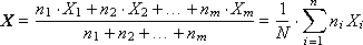
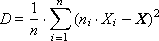
Method 1. Calculate all statistics at the end. To do this, in the course of the experiment, the values ​​of X _{i the} output (studied) random variable X are accumulated in the data array. After the end of the experiment, the expectation (average) X and the variance D (the characteristic variation of the values ​​relative to this expectation) are calculated.

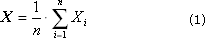
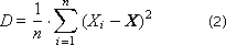
Often, the standard deviation σ = sqrt ( D ) is used.

Note that the disadvantage of the method is the inefficient use of memory, since it is necessary to accumulate and save a large number of values ​​of the output value during the whole experiment, which can be very long.

The second minus is that you have to read the array X _i twice, because using formula (2) as it is written here, we can only calculate the formula (1) (from 1 to n ), and then again banishing for the formula (2) the array X _i .

A positive point is the preservation of the entire data set, which makes it possible to study it in more detail later if necessary to investigate certain effects and results.

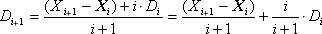
Method 2. Calculation of all statistics in the calculation process (by recursive relations). This method provides the ability to store only the current value of the mathematical expectation X _i and the variance D _i corrected at each iteration. This saves us from the need to permanently store the entire array of experimental data. Each new Xi given is taken into account in the sum with a weighting factor - the more i terms accumulated in the Xi amount, the more important its value is relative to the regular amendment Xi , therefore the ratio of the weighting factors i / ( i + 1): 1 / ( i + 1).

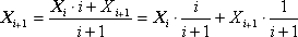
where X _i is the next value of the experimental output value.

Method 3. Calculation of all statistics in class intervals. This method assumes that not all values ​​of X _i will be accumulated in the array, but only over significant intervals in which the random output value X _i is distributed. The total interval of change of X _{i is} divided into m subintervals, in each of which the number n _i is recorded, which indicates how many times X _i took a value from the i -th interval. With a small number of intervals ( m ≈ 1) we get method 1, with the number of intervals m = n we get method 2. In case 1 < m < n, we get an average solution - a compromise between the memory occupied and the information content of the output data.

Distribution geometry calculation

Even more informative is the calculation of the geometry of the distribution of a random variable. It is necessary in order to imagine more accurately the nature of the distribution. It is known that the value of the statistical moment can be approximately judged on the geometric form of the distribution.

The first moment (or arithmetic average) is calculated as follows:

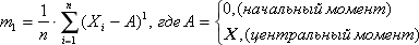
If A takes the value 0, then the first moment is called the initial moment, if A takes the value X , then the first moment is called central. (In principle, A can be any number given by the researcher.)

In practice, it is customary to use not the first moment itself, but its normalized value R ₁ = m ₁ / σ ¹ .

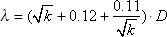
The first moment indicates the center of gravity in the geometry of the distribution, see fig. 34.1.

Fig. 34.1. Characteristic position of the first moment on the graph of statistical distribution

The second moment (or variance, scatter) is calculated as follows:

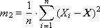
You are familiar with the concept of standard deviation associated with the second point:

In practice, it is customary to use not the second moment itself, but its normalized value R ₂ = m ₂ / σ ² .

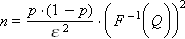
Dispersion characterizes the magnitude of the spread of experimental data relative to the center of gravity m ₁ . Thus, by the value of m ₂ it is possible to judge the second parameter of the geometry of the distribution (see. Fig. 34.2).

Fig. 34.2. Characteristic change in the type of statistical distribution magnitude depending on the magnitude of the second moment

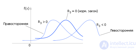
The third moment is characterized by asymmetry (or skewness) (see. Fig. 34.3) is calculated as follows:

In practice, it is customary to use not the second moment itself, but its normalized value R ₃ = m ₃ / σ ³ .

Fig. 34.3. Characteristic change in the type of statistical distribution magnitudes depending on the magnitude of the third moment

By determining the sign of R ₃ , it is possible to determine whether the distribution has asymmetry (see Fig. 34.3), and if there is ( R ₃ ≠ 0), then in what direction.

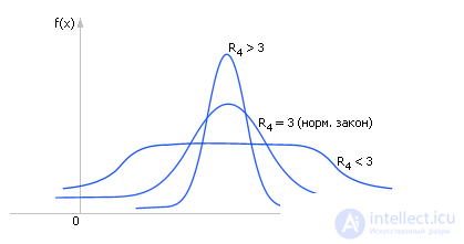
The fourth moment (see fig. 34.4) characterizes the excess (or peakedness) and is calculated as follows:

The normalized moment is: R ₄ = m ₄ / σ ⁴ .

Fig. 34.4. Characteristic change in the type of statistical distribution magnitudes depending on the magnitude of the fourth moment

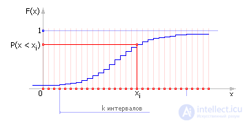
It is very important to find out which distribution most closely resembles the obtained experimental distribution of a random variable. The assessment of the degree of coincidence of the empirical distribution law with the theoretical one is carried out in two stages: the parameters of the experimental distribution are determined and then, according to Kolmogorov, the experimental distribution of the theoretical distribution is assessed.

The estimate (according to Kolmogorov) of the coincidence of the empirical distribution law with the theoretical

1. We calculate the moments m ₁ , m ₂ , m ₃ , ... The number of moments is equal to the number of unknowns in the theoretical distribution law.
2. First of all, since the evaluation concerns a continuous distribution, and we are dealing with a discrete distribution, taken experimentally, then it is necessary to decide how many intervals the sample should be split when sampling.
   
   For this, it is recommended to use the Sturges rule, which has proven itself in practice: K = 1 + log ₂ n = 1 + 3.322 · log ₁₀ n , where n is the number of random values ​​(experiments), k is the number of distribution intervals.
3. An integral (see Fig. 34.5) law is constructed for the empirical distribution F ( x ) = P ( x ≤ x _i ).

   Fig. 34.5. Integral law of empirical distributions, discrete variant (example)

4. Depending on the number of experiments n and the number of intervals 1 ≤ i ≤ k, you can count the number of outcomes in each of the intervals: N _i = Pi + n .
5. Next, you should calculate the theoretical frequency distribution: N _i ^TEOR. = P _i · n . If as a theoretical one we take the normal law of distribution, then we can do this:

   

   where F is the Laplace function, and the parameters a and σ of the law are calculated in Section 1.
6. Compare the obtained frequencies: N _i ^THEOR. and N _i in all k intervals (see fig. 34.6) and choose the greatest deviation of the experimental distribution from the theoretical one being tested:

   

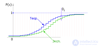
   Fig. 34.6. Comparison of theoretical and empirical integral distributions of a random variable (discrete option)

7. The Kolmogorov parameter λ characterizes the deviation of the theoretical distribution from the experimental one:

   

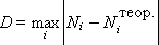
Next, using the table. 34.1 Kolmogorov, should accept or reject the hypothesis of whether the empirical distribution with a given probability Q is theoretical or not. To accept the hypothesis should be: λ < λ _table. .

Note Kolmogorov's criterion is not the only one that can be used for evaluation You can use the Chi-square criterion, the Anderson-Darling criterion and others.

Evaluation of the accuracy of static characteristics

The crucial question is how many experiments should be done so that you can trust the captured characteristics. If the experiments are not enough, then the characteristic is unreliable. Typically, the researcher sets the confidence level, that is, the probability with which he is willing to trust the captured characteristics. The more confidence is given, the more experiments will be required. Previously, we used other methods for estimating the required number of experiments (see Lecture 21, an example of a coin).

So now our estimate will be based on the central limit theorem (see Lecture 25, which states that the sum (or average) of random variables is non-random. The CLT claims that the values ​​of the statistical characteristic we calculate will be distributed according to the normal law, n _i is the number i-th outcomes of the values ​​of the statistical characteristics in n experiments, p _i = n _i / n is the frequency of the i- th outcome.

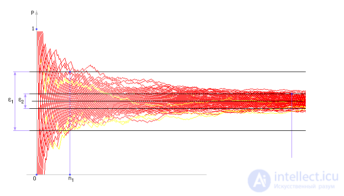
If n -> ∞, then p -> P (the frequency p tends to theoretical probability P ) and the empirical characteristics will tend to theoretical (see. Fig. 34.7). So, according to the CLT, p will be distributed according to the normal law with the expectation m and the standard deviation σ .

Moreover, m = P , σ = sqrt ( p · (1 - p ) / n ).

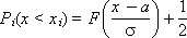
Let Q be the confidence probability , that is, the probability that the frequency p differs from the probability P by no more than ε . Then, by the Bernoulli theorem:

The value of ε is called the confidence interval. The meaning of ε is that in the series (each by sample n ), on average, ε · 100% confidence intervals contain the true value of the statistical characteristic p . As before (see Lecture 25), F is an integral of the function of the normal distribution law, an integral function of Laplace.

Fig. 34.7. Illustration for calculating the number of experiments in magnitude confidence interval according to the central limit theorem

From here we can express the number of experiments required for a confidence probability ( F ^–1 is the inverse Laplace function):

Example. When modeling an enterprise’s products as a result of imitating its work, the following output data were obtained for 50 days (see Table 34.2).

That is, the total was carried out: 15 + 10 + 5 + 20 = 50 experiments ( n = 50). From the table of experiments, the answer of the problem follows, that the frequency (probability) of the release of products of grade 1 is 15/50, the frequency (probability) of release of products of grade 2 is 10/50, the frequency (probability) of release of products of grade 3 is 5/50, the frequency (probability a) release of products 4 grade equal to 20/50.

Let us set the confidence probability for the model answers Q = 0.9 and the confidence interval ε = 0.05.

Now we have to answer the question: is it possible to trust the calculated answer with probability Q ?

We will evaluate the result of statistical experiments according to the worst probability, such in our problem is p = 0.4, since the probability, for example, 0.1 is much better defined.

Very important note . In general, the probabilities (particulars) close to 0 or 1 are very attractive as an answer, since they completely determine the solution. Probabilities close to 0.5 indicate that the answer is very uncertain, the event will happen "50 to 50". It is difficult to call such an answer satisfactory, it is not very informative.

Formula

after substituting the values ​​of F ^–1 (0.9) = 1.65 (see the Laplace table), then ( F ^–1 (0.9)) ² = 2.7, p = 0.4, ε = 0.05 gives N = 0.4 · 0.6 · 2.7 / 0.05 ² or finally N = 250.

That is, our experiment and its answer is unreliable with respect to given Q and ε : 50 experiments are not enough to answer, 250 are required. That is, it is necessary to continue the experiments and conduct 200 more experiments to achieve the required accuracy.

Very important note . The formula uses itself recursively. It is not possible to immediately calculate the number of experiments with it. To calculate n , it is necessary to conduct a test series of experiments, estimate the value of the desired statistical characteristic p , substitute this value in the formula, and determine the necessary number of experiments.

For certainty, this procedure should be carried out several times with different values ​​of n obtained successively.

So, in the block of reliability assessment (AML) (see lecture 21), the degree of reliability of statistical experimental data taken from the model is analyzed (taking into account the accuracy of the result Q and ε given by the user) and the number of statistical tests required for this is determined n .

With a large number of experiments n, the frequency of occurrence of an event p , obtained experimentally, tends to the value of the theoretical probability of occurrence of an event P. If the fluctuation of the frequency of occurrence of events relative to the theoretical probability is less than the specified accuracy, then the experimental frequency is accepted as an answer, otherwise the generation of random input actions is continued, and the simulation process is repeated. With a small number of tests, the result may be unreliable. But the more trials, the more accurate the answer, according to the central limit theorem. The number of required experiments n are given for comparison in Table. 34.3 and tab. 34.4 with various combinations of p and ε .

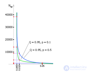
In fig. 34.8 the graph of dependence n ( ε ) is displayed at Q = 0.95 and p = 0.5.

Fig. 34.8. The dependence of the number of required experiments on the value of the confidence probability ε and the confidence interval Q for the case of a frequent occurrence of a random event p = 0.5

Important : evaluation is carried out at the worst of frequencies. This provides a reliable result at once on all the removed characteristics of the model.

Note It should be borne in mind that this estimate of the number of CCT experiments is not the only one existing. There are similar analogous estimates of Bernoulli, Muavre-Laplace, Chebyshev.

How to explain why the curve of the experimentally removed statistical characteristic behaves so strangely (see Fig. 34.7 and Fig. 34.8)? For large n, the curve very slowly approaches the true value, although at first (for small n ) the process proceeds at high speed — we quickly enter the region of an approximate answer (large ε ), but slowly approach the exact answer (small ε ).

For example, suppose we conducted N tests. The fallout of the event in these tests amounted to the number N ₁ . Let the probability of occurrence of an event be close to N ₁ / N = 0.5 or N = N ₁ · 2.

Suppose we want to conduct another test ( N + 1) -e. Taking the answer (frequency N ₁ / N ) with N for 100%, let us estimate how much the percentage will change the answer after the next experiment? Make up the proportion:

N ₁ / N - 100%
( N ₁ + 1) / ( N + 1) - X %

From here we have: X = ( N ₁ + 1) · 100 · N / ( N ₁ · ( N + 1)), with N ₁ = N / 2 (probability 0.5) we get that X = 100 · ( N + 2) / ( N + 1).

And the value of X forms the series: 150%, 133%, 125%, 120%, ..., 100.1%, ..., ... -> 100%. This means that first the improvement in the response to one additional experiment was 50%, by 2 - 33%, by 3 - 25%, by 4 - 20%, ..., by 100% - by only 0.1%.

It can be seen that the accuracy improvement for each new experiment ( X values) is very good at first, and then insignificant, after 100 experiments this value changes only by a fraction of a percent per one additional experiment! The result: a change in the estimate based on the amount, after a series of experiments, ceases to change strongly !!!

Results It is important .

1. As a response to a statistical experiment, we take the frequency p of the appearance of a certain output event, which is an estimate of the probability. Чем больше экспериментов n , тем ближе частость p к вероятности P , а экспериментальный ответ к теоретическому.
2. Частости p , близкие по значению к 0 или 1, более предпочтительны в смысле информативности, чем частости близкие к 0.5, которые мало информативны и дают максимально неопределенный ответ.
3. В моделировании важной целью является понижение дисперсии ответа, разброса выходной величины модели относительно частости. Действительно, если разброс случайной величины m ₂ мал, то вычисленный ответ достаточно достоверен. Если в ряду случайной величины встречаются значения достаточно удаленные друг от друга (см. рис. 34.2), то m ₂ ' велика, и ответ недостаточно определен.
4. Статистический ответ оценивается не только значениями частости и разброса, но и точностью, роль которой играет доверительная вероятность Q и заданный доверительный интервал ε . Эти величины связаны с разбросом m ₂ .
5. The required number of statistical experiments n depends on the given accuracy ( Q , ε ) and the characteristics of the process (frequency p and scatter m ₂ ). Increased accuracy requirements, poor characteristics significantly increase the cost of researching the model, increasing the number of experiments.