Lecture
As we noted earlier, the intensity of the flow in a certain sense is the mathematical expectation of the number of events per unit of time (the inverse of it indicates the average time between events). The second quantity that characterizes how large the time variation of the arrival of events is relative to the expectation is the variance.
Suppose events in a stream follow exactly one after the other every 12 minutes without deviations. The intensity of this flow will be equal to 5 events per hour. But if events happen randomly, for example, 12 ± 2 minutes, then they will, on average, also give 5 events per hour. For example, in 200 hours there will be 1000 events, the intensity value 1000/200 = 5 events per hour. Therefore, according to this characteristic, flows cannot be distinguished from each other. But it is obvious that the second stream will still be more random than the first. Especially, if in the flow of events will follow each other 12 ± 10 minutes.
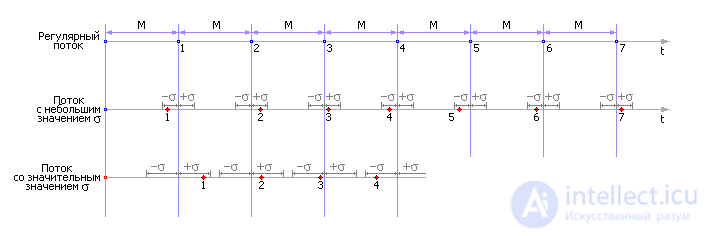
We will call the first stream deterministic, regular, the second and the third random. Moreover, the measure of randomness with increasing dispersion (spread of the interval between events) will increase. In the first stream, the variance is zero. This fact is illustrated in fig. 29.1.
| |
| Fig. 29.1. Illustration of regular and random streams |
Actually, it is the variance that determines the randomness of the occurrence of an event, the weak predictability of the moment of its occurrence. It is important to be able to control this value when modeling random streams. If it is difficult to predict each next event, then the flow is without aftereffect (or with a small aftereffect, there is no connection between events, events are random), if the flow is determined, then the aftereffect is large — each event practically predicts the moment of the next one.
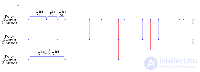
The k- th order Erlang flow is a flow of random events that is obtained if, in the simplest (see Lecture 28) random flow, each kth event is saved and the others are discarded (see Figure 29.2). The flow order is a measure of the flow response. That is, the inverse of the randomness of the flow is its order.
| |
| Fig. 29.2. Illustration of the method of obtaining Erlang streams |
The sifting of events begins to lead to the fact that between the points there is an after-effect, a determination, which is the higher, the larger the k . With increasing k, the points fall on the time axis more and more evenly, their scatter decreases, the regularity increases.
This is based on the simple and previously studied fact that the sum of random variables is a non-random value (the central limit theorem - see Lecture 25). The more random variables we add, the more predictable the result (their sum) will be.
It's obvious that
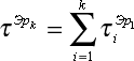
- interval between events in the k- th order Erlang flow.
The probability density of the distribution of intervals between random events in the Erlang flow of the k -th order:
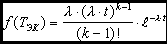
λ k = λ / k is the k- th order Erlang flow intensity, where λ is the intensity of the simplest Poisson flow, and λ k is the intensity of the flow sifted k times, that is, k times less.
The parameters of the Erlang law are calculated by the formulas: M k = 1 / λ k , σ k = 1 / sqrt ( k ) / λ k ,
Note that in the Erlang flow M ≠ σ , that is, in flows with aftereffect, the equality of M and σ is impossible.
Moreover, for k -> ∞, the event occurs strictly in measured time, since σ -> 0.
Compare:
1st order Erlang flow: m = σ 1 - flow without aftereffect;
The Erlang flow of the i- th order: m ≠ σ 2 , with ( σ 2 > 0) and ( σ 1 > σ 2 ), the spread decreases, the after-effect increases;
Erlang ∞-th order flow: m ≠ σ = 0 is a regular flow.
From this it follows that the order of the Erlang flow is a measure of the flow aftereffect.
Example. Consider the example of the failure of light bulbs on a street lighting pole. We take the observation time of 100 years. From the passport data for these products it is known that the average time of the product to failure is 1.5 years; the standard deviation is 0.5 years.
That is, given: M k = 1.5, σ k = 0.5.
Since M k ≠ σ k , then k ≠ 1, that is, we are dealing with a flow with aftereffect. The intensity of this flux is λ k = 1 / M k = 1 / 1.5 = 0.67. The calculated flux rate tells us that during a year, on average, 0.67 light bulbs or 67 light bulbs burn out in 100 years.
Since σ k = 1 / sqrt ( k ) / λ k , and equal to 0.5, then we calculate the order of the Erlang flow: k = 1 / σ 2 / λ k 2 = 1 / 0.5 2 /0.67 2 ≈ 9.
Let us calculate the intensity of the Poisson generating flow λ = λ k · k = 0.67 · 9 = 6.
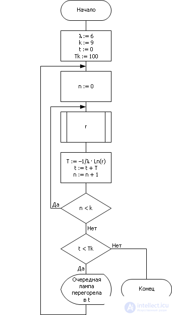
In fig. 29.3 presents an example of an algorithm that implements the modeling of the described process. Note that every ninth event is taken, this ensures a fairly high determinism of the flow (that is, a small dispersion σ k = 0.5).
| |
| Fig. 29.3. Simulation flowchart the appearance of random events in the form of a stream of Erlang |

Comments
To leave a comment
System modeling
Terms: System modeling