Technology using computer models

As we already noted in lecture 01 “The concept of modeling. Ways of presenting models ”, models are built to solve certain problems, so here we look at the types of such tasks and how they use the models that we have already learned how to build.

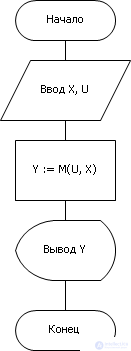
So, the model is a regularity that transforms input values ​​into output: Y = M ( X ). By this we can understand a table, a graph, an expression from formulas, a law (equation), etc. This is a matter of the way in which a pattern is written. In our course and further in the course “Models and Methods of Artificial Intelligence” we will show in detail how to move from one type of record to another.

Under Y in the systems engineering understand some interesting indicator of the researcher or the owner of the system. Each system exists or is created to realize a specific goal. No systems without goals. This is the purpose of the output, the last parameter in the chain of transformations from input to output, which may be of interest to us, since for the sake of it, in fact, all the transformations are done. Those variables that are somehow not connected by circuits with an output indicator do not belong to the system under consideration and must be discarded.

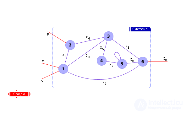
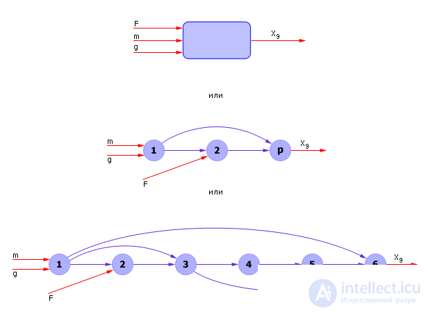
Imagine our system as a graph. This is possible because the system has elements and connections between them, which corresponds to the vertices and arcs of the graph. Further presentation of the material will be based on the example of the graph shown in Fig. 20.1.

Fig. 20.1. Presentation of the system as a graph

The elements of the system are described by laws, that is, equations (variables, operations between them and equalization signs) or systems of equations in the general case, which corresponds to the vertices of the graph. If there are several equations in a vertex, then this vertex can always, if desired, be again divided into a subgraph, where only one equation will already correspond to each vertex. The connections of the graph indicate the connections of the elements of the system among themselves, that is, the connection corresponds to a variable common to two vertices. So, each vertex is associated with a formula (for example, the assignment of an expression or an equation), which associates the variable of the vertex with the other variables that are accessible to it through its connections.

If the graph is sufficiently detailed, such that only one equation corresponds to each vertex, then you can associate vertices with variables. One vertex is one variable. We have already seen the transformed graph in lecture 11. The transition from one form of representation of a graph to another is always possible.

Note: some of the links are inside the graph - these are internal links of the system. Part of the graph links binds the variables of the system X with external variables that are not part of the system, but are part of the environment. These connections cross the boundaries of the graph, the boundaries of the system.

For modeling it is very important to determine where this boundary lies, what will be subject to modeling, and what will not. What will be described by cause-and-effect relationships, and what is not and will remain infinitely large and unknown. Let us once again turn to the text of lecture 01: “...“ Model - search for the finite in the infinite ”- this thought belongs to DI Mendeleev. What is dropped to transform the infinite into the finite? Only essential aspects representing the object are included in the model, and all others are discarded (the infinite majority) ... ”

So, the boundary separates the finite (system) from the infinite (medium). This border can be held in several different places. This suggests that the model can border on several areas that do not have descriptions, which are set in relation to the system only as signals affecting it, as data, but not as laws (see Fig. 1.12). Infinity can also be inside the system, then such a system is called open (see Lecture 11 “Building a model of a dynamic system in the form of differential equations and calculating it by the Euler method”).

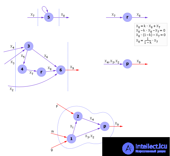
Note that a graph is a strongly related formation, the number of links in such a graph is greater than the number of vertices. In complex systems, links are much larger than vertices. For a normal graph, each vertex must have a connection with any other vertex of the graph through a chain of links. If you find unrelated pieces in the graph, the system model is incorrect or you are dealing with two or more independent systems. If the graph is large, then it makes sense to cut it into small subgraphs and study them separately (see fig. 20.2). It is logical to cut the graph along such lines so that as few links as possible are broken, and as many individual pieces (subgraphs) are obtained. Note that with these actions we, in fact, led the graph to a hierarchical form. Hierarchy is a way of dealing with the complexity of the system being studied. In this case, one vertex is left between the cut lines, the structure of which is decoded separately.

Fig. 20.2. Division of a graph (system) into subgraphs (subsystems)

The application of this technique is very effective if there are several identical subgraphs in the graph. In this case, they are studied separately and once only, and the result is used repeatedly and is generalized to all other cases. Further in the course “Models and Methods of Artificial Intelligence” we will note this technique as basic in human thinking, which is only engaged in building models of objects of the surrounding world in mind, convolving complex constructions into new concepts, solves problems on hierarchical models and struggles thus, with the complexity of the surrounding world.

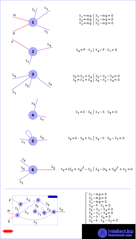
So, the graph defines with its structure the model of the system, which is expressed as a system of interrelated equations (see. Fig. 20.3).

Fig. 20.3. Vertex Matching Illustration a graph describing the subsystems of a large system

Or in the most general form they write:

If among the external variables we determine the goal and define the control (due to which the goal is achieved), then a part of the external variables will be called output variables (target), and another will be called input variables. If an input (control) and an output (goal) are defined on a graph, then the connections of the graph become directed, from input to output (see. Fig. 20.4). These relationships express a causal relationship - changes at the input lead to a change in the values ​​at the output.

Fig. 20.4. Representation of the system as a directed graph, the graph corresponds to a specific problem solved on the system

In this form, the graph corresponds to the problem solved on the graph. The task organizes the order of calculations.

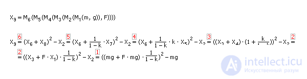
If we now apply successively the equations of the system from the user-assigned input to the output, then from a mathematical point of view, a chain of expressions is formed (see Fig. 20.5). The desired variables will be expressed as a result of the chain through the input variables (see Fig. 20.6). The system of equations by substitution is folded into a formula.

Fig. 20.5. Explicit solution of the problem “Controlling the output of the X 9 system via the input (m, g, F) ​​"by substitution

Fig. 20.6. The procedure for the sequential detail of the graph (operation of composition and decomposition)

In general, it looks like this: Y = M ( M ... ( M ( X )) ...). Such a mathematical structure is called a composition and defines a chain (sequence) of calculations, and therefore an algorithm for calculating the answer of the problem, which in turn determines the solution of the system. The solution can be both numerical and analytical. If the task is different, then the model of the entire system will unfold into another chain, from other input variables to another output. The composition corresponding to the task will change, but the model of the whole system will remain unchanged.

Of course, the chain may not always express the dependence of the output on the input, more often this happens when the input is expressed through the output (input as a function of the output). Expressing the desired through the known, requires the application of inverse to each of the operations applied in the model. For example, the inverse transformation x ₂ = arcsin ( x ₁ ) is applicable to x ₁ = sin ( x ₂ ), the opposite operation x ₂ = sqrt ( x ₁ ) is required to apply to x ₁ = x ₂ ² , and so on. And this is not always possible. It depends on how developed the algebra (transformation rules) of this type of expression. If algebra cannot determine some inverse transformations to a series of expressions, operations, or functions, then the model remains implicit, and special methods for calculating implicit equations must be applied. Solutions in this case are obtained by numerical methods.

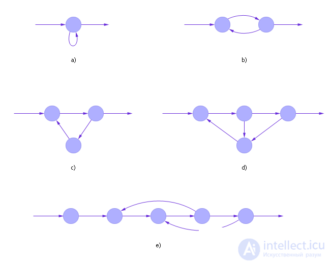
Such complications also come with models containing loops in the graph (see Fig. 20.7).

Fig. 20.7. Examples of graphs of varying complexity containing loops

So, if the input and output are defined and the task is defined on the models, the graph becomes oriented. The task determines the composition of the model, the method of calculating the answer. If the general formula of the system is solved, then the formula is explicit, and the algorithm for its implementation on digital machines will be linear, if there is no analytical solution, then the formula is implicit, and the algorithm will be cyclic.

Now it is time to clarify the concept of input variables, since there are many of them and their list is very heterogeneous. It should be borne in mind that the input variables, which we previously denoted as X , can be denoted for the purposes of detail as X _i , U _i , P _i , Q _i .

First, X may not be a single variable, but an integer vector of variables { X ₁ , X ₂ , ..., X _n }, since the complex systems that we model are usually associated with the environment by many factors { X ₁ , X ₂ , ..., X _n }. Their values ​​are usually of little interest or are not directly accessible to change by the owner of the system, but they exist. Sometimes it is part of the internal variables of the system, state variables, phase variables, system memory, and so on.

Secondly, it is logically convenient to divide the vector X into input variables ( X itself ) and control variables U. Then X is usually understood as factors independent of the will of the system owner, and U as factors that the system owner can directly control at his own will. Such factors are called managed variables or simple control. Note that usually the values ​​of the variables U are somehow limited. In fact, it is impossible to open the water tap by more than 1 (the tap is fully open) or less than 0 (the tap is fully closed). Therefore, if we understand U as the degree of opening of the crane, then 0 ≤ U ≤ 1. In other cases, write a more general version of U _min ≤ U ≤ U _max . In this sense, hereinafter we will assume that management, since it is limited, is a certain resource.

Thirdly, P - slightly changing variables , which in this case are called system parameters; in essence, of course, they differ little from X. In applied tasks, they are often taken out separately, since dynamically they (in the time interval of consideration or existence of the task) do not change and do not change the properties of the system.

Fourth, interference Q. These are variables that act on the system beyond the will of its owner and degrade the value of the desired indicator Y. Interference always acts to the detriment of the owner of the system, understating the desired performance of the system. The control U is a factor that is designed to compensate for the negative effect of interference Q on the output goal indicator Y. That is, with the same value of U , under the action of interference, in contrast to the case of their absence, the indicator Y will be lower. In general, it is often not possible to eliminate all interference to the object for three reasons listed below.

1. The interference acts ahead of the schedule, faster than we can compensate for it, since it is difficult to predict the interference and bring the corresponding control under this beforehand (although sometimes this can be done by special methods of prediction and advance).
2. Interference usually operates rarely, but in large quantities (large amplitude), and there is usually not enough control resource to compensate for it immediately. By the way, it is costly to keep a large supply of control for possible large interference wherever they may occur, since such a resource is deadly capital (non-profitable costs). That is why in large systems there are "black-out", cascading failures and outages, disasters. Managing resource is usually stored in one place and try to deliver it as soon as possible to the place of interference or places where deviations caused by them have already formed. In addition, the effect is caused by rare coincidences of several interferences, which themselves are not catastrophic.
   
   The case when the disturbance acts often (always) and little by little also exists and is well compensated by control (astatic systems).
   
   The case when the obstacle acts over and over and often is incredible, since it must be admitted that in this case the system is poorly designed, and it must simply be redesigned, and not managed.
   
   The case when the disturbance acts rarely and little by little is trivial and simple to control or comes down to the previous versions as a particular one.
3. Interference often arises not where it was waited for and where a resource is located sufficient to compensate for it.

Therefore, they often struggle not with the interference, but with deviations of the variables X and Y from their ideal planned values, struggle with the consequences of accidents, and not with their causes.

Let's move away for a minute from a serious conversation and explain an important point on a comic example. "In order for the cow to give more milk and eat less, it needs to be milked more and fed less." The author of this phrase is the famous showman Nikolai Fomenko (“Russian Radio”). The example demonstrates a fairly common mistake when an engineer confuses and thinks that X = - U (to remove the interference, you must send a compensating signal of the same magnitude and a tighter variable), which is almost impossible in complex systems. The task of management in this joke is solved too trivially, or, more precisely, it is simply set incorrectly, it is simply absent. The reason for this is the lack of a model M. It simply does not describe the cow as a system, as the hay turns into milk. It is not taken into account that control (hay) cannot be used (delivered to the exit) as a target (milk).

So, by controlling U, it is often possible to reduce the negative effect of interference on the target indicator Y. The control action on the interference is there, but it is implicit, more precisely, the interference Q and the control U act on the indicator Y , and the control is chosen so as to negate the negative effect of interference on Y.

And, of course, it should be remembered that efforts to compensate for interference always cost the system owner something, since they use the same resource, which we designated earlier as U _max . So, note: the concept of a resource is always connected with management. Management draws its strength from the resource. If the resource is small, then the control is connected and cannot cope with strong interference.

If the resource is instantly renewable, then U _min ≤ U ≤ U _max . If the resource has the property of additivity, accumulates and is wasted, can not instantly resume, then

where U _ir ( t ) is the rate of resource use, U _ol ( t ) is the rate of resource supply.

As is well known from mathematics, and was already considered in Lecture 01, with the expression Y = M ( X ), three types of problems can be solved, which are listed in Table. 20.1.

Analysis task (direct problem)

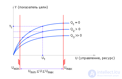
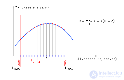
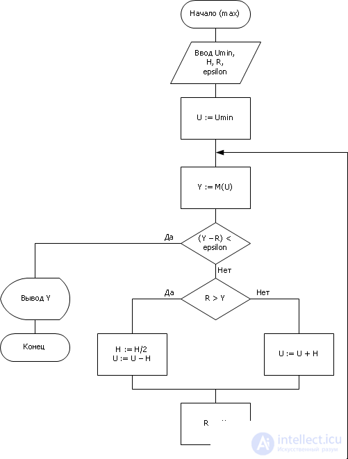
The influence of some input parameter U on the final result or index Y is studied. 1, 2, ..., N - experiments conducted with the model. If we repeatedly supply different values ​​of U to model M (the algorithm is shown in Fig. 20.10), then, by measuring Y , as a result of modeling, we can construct the dependence Y = M ( U ) at the model output, see Fig. 20.8. Usually, they are actually limited to some set of input actions U _min ≤ U ≤ U _max , passing U values ​​point by point with a certain step Δ U. At the same time, during such an experiment, part of the input parameters X is frozen, leaving their values ​​unchanged. If necessary, you can repeat the experiment on the search of U from the interval U _min ≤ U ≤ U _max with a different value of X. In this case, we obtain a family of curves Y = M ( U , X ), see fig. 20.9.

Fig. 20.8. An exemplary view of the dependence of goal Y on control U, obtained experimentally on a system model

Fig. 20.9. Approximate view of dependence of goal Y on control U at various values ​​of effective interference Q

Fig. 20.10. Algorithm used in solving direct model research problem (analysis)

That is, experiencing repeatedly the model with different input signals, we can get the dependence of the output on the input. Such a problem is called direct (see lecture 01). Результатом задачи является кривая, семейство кривых, таблица, а когда это возможно, то формула, закон и т. д. Основной вопрос анализа — познание свойств объекта. «Воздействуем на объект и смотрим, что получится, как он реагирует, делаем вывод о его свойствах, возможностях».

Important! Важными понятиями в системотехники являются «управляемость» и «наблюдаемость» . По виду кривых Y = M ( U ) (рис. 20.9) можно определить, для всех ли значений Y возможно некоторое значение входного сигнала ( U , X )? Любое ли значение Y можно достигнуть, используя переменные( U , X ) из выбранного диапазона. То есть характер кривых указывает, в какой области Y объект является управляемым. Понятие «управляемость» касается выходной переменной.

Наблюдаемость — возможность измерения, анализа той или иной характеристики объекта. Иногда из-за того, что некоторая величина не может быть непосредственно измерена в результате эксперимента, приходится, чтобы получить о ней хоть какое-то представление, довольствоваться косвенными показателями. Понятие «наблюдаемость» касается выходной переменной. Проектировать системы надо так, чтобы качество наблюдаемости и управляемости были обеспечены.

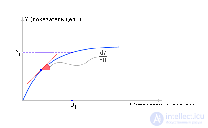
Отношение изменения Y к изменению U (при фиксированном X ) называется чувствительностью Y по U . Обычно, так как кривая Y = M ( U ) для сложных систем нелинейна, то изменение U принимают небольшой величиной, в идеале Δ U –> 0. В математическом смысле, чувствительность — это производная d Y /d U . Понятие чувствительности касается отношения выхода ко входу (рис. 20.8).

To reduce the number of tests, the input effects are chosen according to a certain rule. Naturally, the desire to obtain the necessary amount of information about the system with a minimum number of tests. Such a test system is planned by a factor experiment.

Synthesis task (inverse problem)

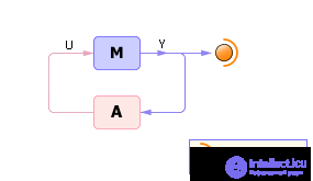
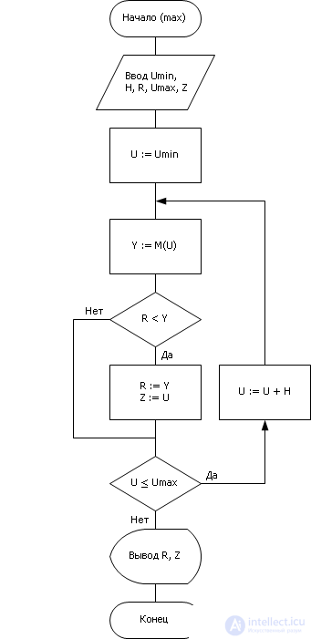
Цель задачи синтеза — нахождение экстремума функции результата. Когда анализ закончен и построены функции, графики, таблицы, когда объект (его свойства и поведение) исследован во всех вариантах возможных входных воздействий, имеет смысл найти среди всего этого многообразия откликов наилучший. Обычно выход — цель функционирования системы, и логично принять, что цель должна принимать лучшие из всех возможных значений, потому имеет смысл найти такие значения входных параметров U , при которых выходной показатель Y примет свое наилучшее значение (экстремум). При этом под экстремумом может подразумеваться как минимум, так и максимум зависимости Y ( U ). Чтобы найти экстремум, модель включают в контур (см. рис. 20.11) с некоторым алгоритмом A , осуществляющим автоматическое управление входом U и построенным так, что в результате его работы производится поиск такого входного воздействия U на модель M , при котором она выдает наилучший выходной результат.

Fig. 20.11. Схема решения обратных задач (синтез)

Существуют различные алгоритмы поиска оптимума функции Y = M ( U ). Упомянем три из них (подробно эти и другие методы вы будете изучать в дисциплине «Системный анализ и исследование операций»).

1. Метод перебора. Алгоритм метода перебора представлен на рис. 20.12. Этот метод обеспечивает поиск глобального экстремума, но расточителен к вычислительным ресурсам, так как просматривает все возможные входные значения U с определенным шагом H и выбирает наилучший среди всех выходных результатов Y (см. рис. 20.13). Наилучшее из встреченных Y сохраняется и уточняется в ячейке R , значение U при этом значении Y сохраняется по ходу алгоритма в ячейке Z . Кроме этого имеется риск пропустить нужную точку, «перешагнув» через нее из-за слишком большого размера шага H .
   
   

   Fig. 20.12. Алгоритм перебора, примененный к решению задачи синтеза — поиск наилучшего U для максимизации Y

   Fig. 20.13. Характерный рисунок поиска экстремума функции Y = M(U) методом перебора

2. Метод деления шага пополам. Этот метод более экономичен по отношению к методу перебора, так как анализирует по ходу движения, в каком направлении происходит улучшение (увеличение или уменьшение) функции Y = M ( U ) и старается двигаться именно в этом направлении. Если при этом попутно обнаруживается, что тенденция во время движения изменилась (уменьшение Y сменилось на его увеличение или наоборот), то алгоритм (рис. 20.14) разворачивается обратно (то есть меняет знак приращения входного сигнала на обратный) и снова идет в нужную сторону, но шаг при этом уменьшается вдвое. Это позволяет подойти к точке экстремума с малым значением шага поиска, что лучше локализует результат (см. рис. 20.15).

   Fig. 20.14. Алгоритм деления шага пополам, примененный к решению задачи синтеза — поиск наилучшего U для максимизации Y

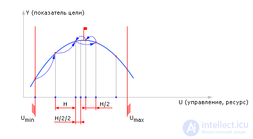
   Fig. 20.15. Характерный рисунок поиска экстремума функции Y = M(U) методом деления шага пополам

3. Метод градиента. Метод, алгоритмическая реализация которого представлена на рис. 20.16, использует свойства гипотетической кривой Y = M ( U ), а именно тот факт, что по направлению производной p , вычисленной на основе двух рядом стоящих точек, можно определить, в какую сторону уменьшается (увеличивается) значение цели Y и двигаться сразу в нужную сторону (см.рис. 20.17). Такая стратегия существенно сокращает время поиска. Недостатком алгоритма является то, что производная может перестать меняться в области локального экстремума, и глобальный экстремум такой алгоритм не найдет.

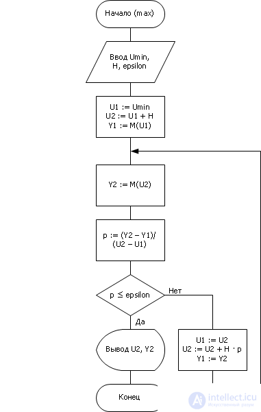
   Fig. 20.16. Алгоритм поиска экстремума методом градиента, примененный к решению задачи синтеза

   Fig. 20.17. Характерный рисунок поиска экстремума функции Y = M(U) методом градиента

Задачу настройки модели мы уже подробно обсуждали в лекциях 02—08 (см. лекцию 02), и останавливаться на ней мы уже не будем. Это способы построения собственно самой модели.

Simulators

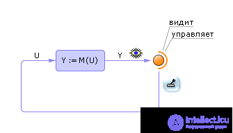
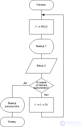
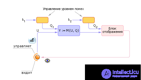
Этот класс задач, использующих модели, применяют для выработки навыков обучения у управляющего персонала. К тренажерам близки компьютерные игры. Управление моделью в данном случае осуществляет человек-оператор, который наблюдает за выходом модели (см. рис. 20.18). Воздействуя на вход модели, оператор старается добиться нужного выходного результата, и в процессе этих действий получает необходимые навыки по управлению, которые затем может перенести на реальный объект. In fig. 20.19 показан примерный вид алгоритма реализации тренажера на базе модели.

Fig. 20.18. Схема использования модели в тренажерах

Fig. 20.19. Типичный вид алгоритма реализации тренажера

Разумеется, тренажер должен обладать качествами наблюдаемости и управляемость. То есть оператор в принципе может и должен судить о качестве своих действий, только наблюдая какие-то важные для себя результаты на выходе. И модель должна быть построена таким образом, чтобы можно было достичь хотя бы в принципе искомых результатов какими-то входными воздействиями на нее (управляемость).

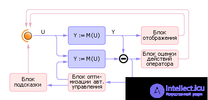
Параллельно с моделью может функционировать система оценки деятельности оператора, а также блок автоматического определения наилучших решений, которые могут в определенных режимах (например, режим обучения или подсказки) помогать оператору (см. рис. 20.20). Для этого к модели следует подключить экспертную систему, дающую рекомендации оператору в затруднительных для него случаях.

Fig. 20.20. Схема построения тренажера с функциями экспертной системы

Для выработки устойчивых навыков у персонала в процессе тренажа в информацию вносят дополнительные помехи, имитирующие реальные сложности, возникающие на объекте. Можно вносить помехи на входе (нарушается управляемость), на выходе (нарушается наблюдаемость) или в переменные состояния модели (см. рис. 20.21). Следует различать равнодушно действующие помехи и целенаправленное противодействие. В первом случае речь идет о случайном процессе, мешающем оператору достичь цель. Случайная помеха может, как увеличить свое значение, так и равновероятно уменьшить его, то есть чаще всего среднее значение помехи на большом интервале времени равно нулю. Во втором случае речь идет о целенаправленной дезинформации оператора (среднее ее действия не равно нулю).

Для тренажа играет большую роль среднее значение и дисперсия величины помех, которые постепенно наращивают с ростом опыта оператора.

Fig. 20.21. Схема тренажера, дополненного генератором помех

Теперь обсудим вопросы снятия и использования системных характеристик, то есть таких характеристик, которые представляют свойства системы в целом. Напомним, важнейшими понятиями для системы являются управление, помехи, цель. Системная характеристика должна связать эти понятия вместе. Методика снятия характеристик такова.

Select the variables U (input, control) and Y (output, target) for the study.

We fix the remaining X as some fixed value. For each U from the range of permissible values U _min ≤ U ≤ U _{max we} observe and fix in the table. 20.2 Y result.

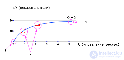
On the graph (see fig. 20.22) we build a point with coordinates ( U , Y ). As a result of a series of experiments, the Y ( U ) curve is obtained, which shows the dependence of the output on the input, on the target, on the control.

Usually, if we are dealing with a model reflecting a complex system, it is quite real, with a high degree of adequacy, the dependence Y ( U ) should have approximately the same dependence, as shown in Fig. 20.22.

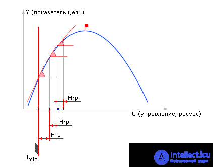
Fig. 20.22. Approximate view of goal indicator dependency from control (resource) characteristic of complex systems

ATTENTION! Here are the most common arguments, the type of curve can be quite different !!!! In fig. 20.22 clearly visible the following patterns.

1. The curve comes from zero. If you don’t manage it, don’t invest a resource, don’t try, the system itself is unlikely to produce the result you need, which is useful to you.
2. The curve is non-linear. At first (for small values ​​of U ), even small efforts apply to a good increase in the target indicator. Then (for large values ​​of U ) each successive succession Δ Y is given by an increasing effort Δ U. Mathematically speaking, at first with small U , the derivative Δ Y / Δ U is of great importance, with increasing U its value decreases.
3. The curve has a fading character, tends to saturation. Indeed, imagine if you invest enormous values ​​of a resource (for example, spend a billion rubles on advertising your gas station in Perm), you are unlikely to receive a corresponding profit. The profit Y on this section U will be limited by other factors (the presence of those who want to refuel will be no more than the number of car owners in the city, for example). The real system sooner or later, but goes to a certain "limit", the "emphasis", saturation.

Select a variable Q in the object. In the sense of this variable should prevent to reach the goal and not depend on the will of the owner, he can not manage it.

Next, you should change the value of Q (previously we thought it was 0) and carry out all the above steps again (see table. 20.3).

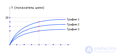
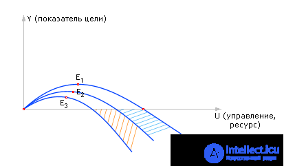
And again build on the table of experiments schedule (see. Fig. 20.23). Obviously, under the action of disturbances Q, graph 2 will be lower than graph 1, since the presence of interference means that more control efforts U must be applied to achieve the same effect Y. Note that it is not necessary to change Q during U change in order to clearly see the connection of Y precisely from U.

Fig. 20.23. Approximate view of the dependence of the target indicator from control (resource) and disturbances characteristic of complex systems

Important!!! If the interference is still spontaneously changing during the removal of the Y ( U ) curve, and this happens when the interference is random, then you should first apply several experiments with the same U and then average the result of y . The average value is more reliable than one of the random implementations. How many experiments need to be conducted for averaging to ensure the specified accuracy of the answer, we will discuss with you later in lecture 21 and lecture 34.

Increase Q again and perform experiments again, and again get a new table (see table. 20.4) and a new graph (see fig. 20.23) - Y ( U ). As a result, you get a family of curves 1-2-3, reflecting the dependence of the target, both on the control and on the interference.

The removal of experimental data is completed. Now, at any time with given Q and Y , using graphs 1, 2, 3, you can predict the result - the level of control U that is necessary to achieve the goal Y. Such a task, we recall, is called the inverse.

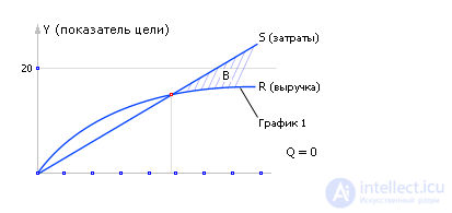
Now, using the removed dependencies, it is useful to find the best solutions among the many possible. To do this, on each chart 1, 2, 3 we will additionally build the cost line S (spending), since management is always worth something, and the more you use this resource, the more you have to pay for it. The slope of this line indicates the price of the resource (see fig. 20.24).

Fig. 20.24. Combined schedules of sales revenue goal (revenue) and the cost of achieving it

Let us take, for example, that the price of a resource is unchanged and does not depend on how much you use it (although, we note that there are wholesale discounts).

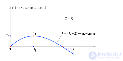
Suppose we have to maximize goal Y. Then the curve R (receipts), expressed in value units, symbolizes revenue, and the line S (spending), expressed in the same value units, symbolizes expenses. If we subtract costs from revenues, that is, we subtract one point from another point by point ( R - S ), then we end up with a profit P (profit): P = R - S. Namely, how profit depends on management (see. Fig. 20.25).

Fig. 20.25. The summary schedule of the profit received (revenue minus costs) depending on the size of the control (resource) U. The best solution - maximum profit - point E 1 , best management - U 1

Obviously, zone B (bankrupt) is a bankruptcy zone, point N (null) is the point “do nothing and have nothing” and point E ₁ (extremum) is the zone of the greatest profit. To get profits more than Y ₁ at this level, interference Q will not succeed. This point symbolizes the simple fact that the result achieved at any cost does not pay back the excessive efforts to achieve it, “everything is good in moderation”. Any control actions, even larger than U ₁ , give the worst result .

Similarly, we find the point E on the remaining graphs 2, 3 - E ₂ , E ₃ .

Fig. 20.26. Graphs of profit, depending on the amount of control (resource) U and perturbations Q. Points of best solutions Е i - maximum arrived. Best management appropriate to them - U i

Let's reduce all points E from all three graphs to one new graph (see fig. 20.27).

Fig. 20.27. Final Schedule for Best Solutions E according to the criterion of profit Y depending on the size control (resource) U and disturbances Q

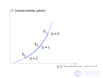
We have obtained a remarkable dependence “the curve of optimal values ​​of the goal Y depending on the best solutions U at a given level of interference Q ”, from which one can find the optimal applied control efforts necessary to achieve the best result in these conditions. Let's call this curve the “interdependence of purpose, control, and interference.”

The graph shows that the largest attainable possible profit decreases from point to point with increasing magnitude of interference - point E shifts. For example, it is possible that the interference is very strong, and the resource has a fixed price, then it is possible that it is better not to do anything.

Taking into account the above and returning to lecture 01 (Fig. 1.9—1.10), we once again note that building and using models as part of software products is a promising new direction in software design. The study of optimal options for enterprise management should be provided with modeling tools.