Lecture
A large class of systems that are difficult to study by analytical methods, but which are well studied by statistical modeling methods, are reduced to queuing systems (QS).
The QS implies that there are typical paths (service channels) through which applications are processed during processing. It is customary to say that applications are served by channels. Channels can be different in purpose, characteristics, they can be combined in different combinations; applications can be in queues and wait for service. Some applications may be served by channels, and parts may refuse to do so. It is important that the application, from the point of view of the system, are abstract: this is what wants to serve, that is, to go a certain way in the system. Channels are also an abstraction: this is what serves applications.
Applications may arrive unevenly, channels may serve different applications at different times, and so on, the number of applications is always very large. All this makes such systems difficult to study and control, and it is not possible to trace all the causal relationships in them. Therefore, the notion that service in complex systems is random is accepted.
Examples of SMOs (see table. 30.1) are: bus route and passenger transportation; production conveyor for parts processing; a squadron of aircraft flying into foreign territory, which is “serviced” by air defense anti-aircraft guns; barrel and horn of the machine, which "serve" the cartridges; electric charges moving in some device, etc.
| Table 30.1. Examples of queuing systems | ||||||||||||||||||
|
But all these systems are combined into one class of QS, since the approach to their study is one. It consists in the fact that, firstly, random numbers are played with the help of a random number generator, which imitate the RANDOM moments of the appearance of requests and the time they serve in the channels. But in aggregate, these random numbers, of course, are subject to statistical laws.
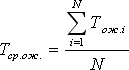
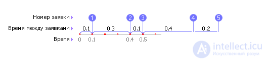
For example, let it be said: “applications on average come in the amount of 5 pieces per hour.” This means that the times between the arrival of two neighboring orders are random, for example: 0.1; 0.3; 0.1; 0.4; 0.2, as shown in Fig. 30.1, but in total they give an average of 1 (note that in the example it is not exactly 1, but 1.1 - but in another hour this amount, for example, can be equal to 0.9); and only for a sufficiently long time, the average of these numbers will become close to one hour.
| |
| Fig. 30.1. The random process of the arrival of applications in the QS |
The result (for example, the capacity of the system), of course, will also be a random variable at separate intervals of time. But measured over a large period of time, this value will already, on average, correspond to the exact solution. That is, to characterize the QS are interested in the answers in a statistical sense.
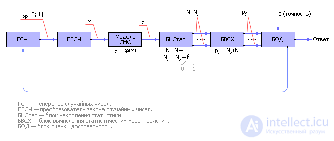
So, the system is tested with random input signals subordinate to a given statistical law, and as a result they take statistical indicators averaged over the time of consideration or the number of experiments. Earlier, in Lecture 21 (see Fig. 21.1), we have already developed a scheme for such a statistical experiment (see Fig. 30.2).
| |
| Fig. 30.2. Statistical experiment scheme for studying queuing systems |
Secondly, all models of QS are collected in a typical way from a small set of elements (channel, source of applications, queue, application, service discipline, stack, ring, and so on), which allows you to simulate these tasks in a typical way. For this, the system model is assembled from the designer of such elements. No matter what specific system is being studied, it is important that the scheme of the system is assembled from the same elements. Of course, the structure of the scheme will always be different.
We list some basic concepts of QS.
Channels are what they serve; there are hot (starting to serve the application at the moment it enters the channel) and cold (the channel to start servicing takes time to prepare). Application sources - generate applications at random times, according to the statistical law specified by the user. Applications, they are clients, enter the system (generated by the sources of applications), pass through its elements (served), leave it served or unmet. There are impatient applications - those that are tired of waiting or being in the system and who leave of the QO of their own accord. Requests form streams - the flow of requests at the input of the system, the flow of served requests, the flow of refused requests. A flow is characterized by the number of applications of a certain grade observed in a certain place of the QS per unit of time (hour, day, month), that is, the flow is a statistical value.
Queues are characterized by the rules of standing in a queue (service discipline), the number of places in a queue (how many clients can be in a queue at most), the structure of a queue (connection between places in a queue). There are limited and unlimited queues. We list the most important disciplines of service. FIFO (First In, First Out - first came, first left): if the application came first in the queue, then it will go to the service first. LIFO (Last In, First Out - the last to come, the first to leave): if the application last came in the queue, then it will be the first to be served (for example, the cartridges in the horn of the machine). SF (Short Forward - Short Forward): those applications from the queue that have a shorter service time are served first.
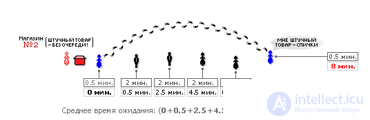
We will give a vivid example showing how the right choice of a particular discipline of service allows you to get tangible savings in time.
Suppose there are two stores. In Shop No. 1, service is carried out in turn, that is, the FIFO service discipline is implemented here (see Fig. 30.3).
| |
| Fig. 30.3. Queuing on FIFO discipline |
Service time t serviced . in fig. 30.3 shows how much time the seller will spend on servicing a single buyer. It is clear that when buying piece goods, the seller spends less time on maintenance than when buying, say, bulk products that require additional manipulations (dial, weigh, calculate the price, etc.). Wait time t wait . shows how long the next buyer will be served by the seller.
The shop number 2 is implemented discipline SF (see. Fig. 30.4), which means that piece goods can be bought out of turn, because the service time t service . such a purchase is small.
| |
| Fig. 30.4. Queuing for the SF discipline |
As can be seen from both figures, the last (fifth) buyer is going to purchase piece goods, so his service time is short — 0.5 minutes. If this buyer comes to the store number 1, he will be forced to stand in line for 8 minutes, while in the store number 2 he will be served immediately, out of turn. Thus, the average service time of each customer in a store with FIFO service discipline will be 4 minutes, and in a store with service discipline KV - only 2.8 minutes. And the public benefit, saving time will be: (1 - 2.8 / 4) · 100% = 30 percent! So, 30% of the time saved for the society is only due to the correct choice of the discipline of service.
A systems specialist should have a good understanding of the performance and efficiency resources of the systems he designs, hidden in the optimization of parameters, structures and maintenance disciplines. Simulation helps to reveal these hidden reserves .
When analyzing the results of modeling, it is also important to indicate the interests and the degree of their implementation. Distinguish the interests of the client and the interests of the owner of the system. Note that these interests do not always coincide.
Judging the results of the QS can be indicators. The most popular of them are:
It is necessary to judge the quality of the resulting system by the totality of the values of the indicators. When analyzing the results of modeling (indicators), it is also important to pay attention to the interests of the client and the interests of the owner of the system, that is, one or another indicator must be minimized or maximized, as well as the degree of their fulfillment. Note that most often the interests of the client and the owner do not coincide with each other or they do not always coincide. Indicators will be denoted below H = { h 1 , h 2 , ...}.
The parameters of the QS can be: the intensity of the flow of requests, the intensity of the service flow, the average time during which the application is ready to wait for service in the queue, the number of service channels, the discipline of service, and so on. Parameters - this is what affects the performance of the system. The parameters will be denoted below as R = { r 1 , r 2 , ...}.
Example. Gas station (gas station).
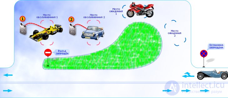
1. Statement of the problem . In fig. 30.5 shows the plan of the gas station. Consider the method of modeling the QS by its example and the plan for its research. Drivers, driving along the road past the gas station along the road, may want to refuel their car. They want to be serviced (fill the car with gasoline) not all motorists in a row; Let us assume that, on average, out of the total flow of cars, 5 cars per hour enter a gas station.
| |
| Fig. 30.5. Simulated gas station plan |
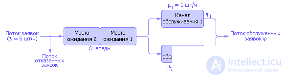
At the gas station two identical columns, the statistical performance of each of which is known. The first column serves on average 1 car per hour, the second on average - 3 cars per hour. The owner of the gas station has asphalted a place for cars where they can expect service. If the speakers are busy, then other cars can expect service at this place, but no more than two at a time. The queue will be considered common. As soon as one of the columns is free, the first car from the queue can take its place on the column (while the second car moves to the first place in the queue). If a third car appears, and all the places (there are two of them) in the queue are occupied, then they are denied service, as it is prohibited to stand on the road (see traffic signs near the gas station). Such a machine leaves the system forever and as a potential customer is lost to the gas station owner. You can complicate the task by considering the cashier (another service channel, where you need to get after the service in one of the columns) and the queue to it, and so on. But in the simplest version, it is obvious that the paths of the flow of applications through the QS can be depicted in the form of an equivalent circuit, and adding the values and designations of the characteristics of each element of the QS, we finally get the diagram shown in fig. 30.6.
| |
| Fig. 30.6. Equivalent schema object modeling |
2. Method of investigation of QS . Let us apply in our example the principle of sequential posting of applications (for details on the principles of modeling, see Lecture 32). His idea is that the application is carried out through the entire system from the entrance to the exit, and only after that they take up the modeling of the next application.
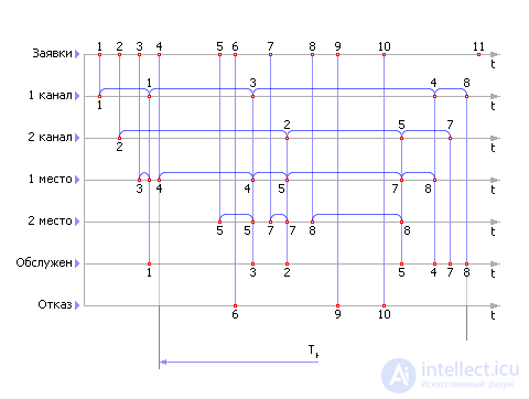
For clarity, we construct a time diagram of the operation of the QS, reflecting on each ruler (time axis t ) the state of a separate element of the system. There are as many time lines as there are different places in the QS, flows. In our example, there are 7 of them (application flow, wait flow in the first place in the queue, wait flow in the second place in the queue, service flow in channel 1, service flow in channel 2, flow of requests serviced by the system, flow of rejected requests).
To generate the arrival time of applications, we use the formula for calculating the interval between the arrival times of two random events (see Lecture 28):

In this formula, the flux λ must be specified (before it must be determined experimentally on the object as a statistical mean), r is a random uniformly distributed number from 0 to 1 from the RNG or a table in which random numbers must be taken in succession (without specifically choosing ).
Task. Generate a stream of 10 random events with an intensity of occurrence of events of 5 pieces / hour.
The solution of the problem. Take random numbers evenly distributed in the range from 0 to 1 (see table), and calculate their natural logarithms (see table. 30.2).
| Table 30.2. Fragment of random table numbers and their logarithms | ||||||||||
|
The formula of a Poisson flow determines the distance between two random events as follows: t = –Ln (r рр ) / λ . Then, given that λ = 5, we have the distances between two random neighboring events: 0.68, 0.21, 0.31, 0.12 hours. That is, events occur: the first at time t = 0, the second at time t = 0.68, the third at time t = 0.89, the fourth at time t = 1.20, the fifth at time t = 1.32 and etc. Events - the arrival of applications reflect on the first line (see. Fig. 30.7).
| |
| Fig. 30.7. Timing diagram of the QS |
The first application is taken and, since at this moment the channels are free, it is set up for service in the first channel. Application 1 is transferred to the line "1 channel".
The service time in the channel is also random and is calculated using a similar formula:

where the role of intensity is played by the value of the service flow μ 1 or μ 2 , depending on which channel serves the application. We find on the diagram the moment of the end of the service, postponing the generated service time from the moment of the beginning of the service, and omit the application for the “Served” line.
The application went to the SMO all the way. Now you can, according to the principle of sequential posting of applications, also simulate the path of the second application.
If at some point it turns out that both channels are busy, then an application should be placed in the queue. In fig. 30.7 is the application with number 3. Note that, according to the conditions of the task, in the queue, unlike the channels, the requests are not random time, but wait for one of the channels to be released. After the channel is released, the application rises to the line of the corresponding channel and its maintenance is organized there.
If all the places in the queue at the time when the next application arrives, will be occupied, then the application should be sent to the “Denied” line. In fig. 30.7 is application number 6.
The procedure for imitation of service applications continue for some time observation T n . The longer this time, the more accurate the simulation results will be in the future. In reality, for simple systems, T n equal to 50–100 hours or more is chosen, although sometimes it is better to measure this value by the number of considered applications.
The analysis will be carried out on the already considered example.
First you need to wait for the steady state. We discard the first four applications as uncharacteristic, proceeding during the process of establishing the work of the system. We measure the observation time, let us assume that in our example it will be T n = 5 hours. Calculate from the chart the number of serviced requests N obs. , idle times and other quantities. As a result, we can calculate indicators characterizing the quality of work of the QS.
Next, you should evaluate the accuracy of each of the results obtained. That is, to answer the question: how much can we trust these values? Accuracy assessment is carried out according to the method described in lecture 34.
Если точность не является удовлетворительной, то следует увеличить время эксперимента и тем самым улучшить статистику. Можно сделать и по-другому. Снова несколько раз запустить эксперимент на время T н . А в последствии усреднить значения этих экспериментов. И снова проверить результаты на критерий точности. Эту процедуру следует повторять до тех пор, пока не будет достигнута требуемая точность.
Далее следует составить таблицу результатов и оценить значения каждого из них с точки зрения клиента и владельца СМО (см. табл. 30.3).. В конце, учитывая сказанное в каждом пункте, следует сделать общий вывод. Таблица должна иметь примерно такой вид, какой показан в табл. 30.3.
| Таблица 30.3. Показатели СМО | |||||||||||||||||||||||||
| |||||||||||||||||||||||||
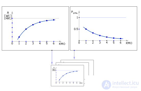
Мы проделали анализ существующей системы. Это дало возможность увидеть ее недостатки и определить направления улучшения ее качества. Но остаются непонятными ответы на конкретные вопросы, что именно надо сделать — увеличивать количество каналов или увеличивать их пропускную способность, или увеличивать количество мест в очереди, и, если увеличивать, то насколько? Есть и такие вопросы, что лучше — создать 3 канала с производительностью 5 шт/час или один с производительностью 15 шт/час?
Чтобы оценить чувствительность каждого показателя к изменению значения определенного параметра, поступают следующим образом. Фиксируют все параметры кроме одного, выбранного. Затем снимают значение всех показателей при нескольких значениях этого выбранного параметра. Конечно, приходится повторять снова и снова процедуру имитации и усреднять показатели при каждом значении параметра, оценивать точность. Но в результате получаются надежные статистические зависимости характеристик (показателей) от параметра.
Например, для 12 показателей нашего примера можно получить 12 зависимостей от одного параметра: зависимость вероятности отказов P отк. от количества мест в очереди (КМО), зависимость пропускной способности A от количества мест в очереди, и так далее (см. рис. 30.8).
| |
| Fig. 30.8. Примерный вид зависимостей показателей от параметров СМО |
Затем так же можно снять еще 12 зависимостей показателей P от другого параметра R , зафиксировав остальные параметры. And so on. Образуется своеобразная матрица зависимостей показателей P от параметров R , по которой можно провести дополнительный анализ о перспективах движения (улучшения показателей) в ту или иную сторону. Наклон кривых хорошо показывает чувствительность, эффект от движения по определенному показателю. В математике эту матрицу называют якобианом J, в которой роль наклона кривых играют значения производных Δ P i /Δ R j , см.рис. 30.9. (Напомним, что производная связана геометрически с углом наклона касательной к зависимости.)
| |
| Fig. 30.9. Якобиан — матрица чувствительностей показателей в зависимости от изменения параметров СМО |
Если показателей 12, а параметров, например, 5, то матрица имеет размерность 12 x 5. Каждый элемент матрицы — кривая, зависимость i -го показателя от j -го параметра. Каждая точка кривой — среднее значение показателя на достаточно представительном отрезке T н или усреднено по нескольким экспериментам.
Следует понимать, что кривые снимались в предположении того, что все параметры кроме одного в процессе их снятия были неизменны. (Если бы все параметры меняли значения, то кривые были бы другими. Но так не делают, так как получится полная неразбериха и зависимостей не будет видно.)
Поэтому, если на основании рассмотрения снятых кривых принимается решение о том, что некоторый параметр будет в СМО изменен, то все кривые для новой точки, в которой опять будет исследоваться вопрос о том, какой параметр следует изменить, чтобы улучшить показатели, следует снимать заново.
Так шаг за шагом можно попытаться улучшить качество системы. Но пока эта методика не может ответить на ряд вопросов. Дело в том, что, во-первых, если кривые монотонно растут, то возникает вопрос, где же все-таки следует остановиться. Во-вторых, могут возникать противоречия, один показатель может улучшаться при изменении выбранного параметра, в то время как другой будет одновременно ухудшаться. В-третьих, ряд параметров сложно выразить численно, например, изменение дисциплины обслуживания, изменение направлений потоков, изменение топологии СМО. Поиск решения в двух последних случаях проводится с применением методов экспертизы (см. лекцию 36. Экспертиза) и методами искусственного интеллекта (см. генетические алгоритмы в искусственном интеллекте.
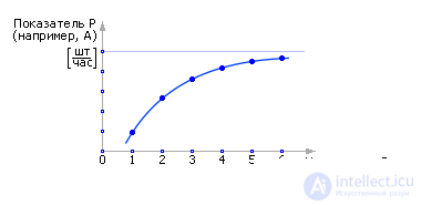
Therefore, now we discuss only the first question. How to make a decision, what should be the value of a parameter, if with its growth the indicator is monotonously improving all the time? It is unlikely that the value of infinity will suit the engineer.
The R parameter is management, this is what is at the disposal of the owner of the QS (for example, the ability to asphalt the site and thereby increase the number of places in the queue, put additional channels, increase the flow of applications by increasing advertising costs, and so on). Changing the control, you can influence the value of the indicator P , the goal, the criterion (the probability of failures, throughput, average service time, and so on). From fig. 30.10 it is clear that if you increase the control of R , then you can always achieve an improvement in the index P. But it is obvious that any control is associated with costs Z. And the more efforts are made to control, the greater the value of the control parameter, the greater the costs. Typically, management costs grow linearly: Z = C 1 · R. Although there are cases when, for example, in hierarchical systems, they grow exponentially, sometimes back exponentially (discounts for wholesale) and so on.
| |
| Fig. 30.10. Dependence of the indicator P from the controlled parameter R (example) |
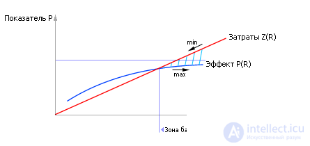
In any case, it is clear that once all the investment of new costs simply cease to pay for itself. For example, the effect of an asphalted site measuring 1 km 2 is unlikely to pay back the costs of the owner of a gas station in Uryupinsk; there simply will not be so many people willing to refuel with gasoline. In other words, the indicator P in complex systems cannot grow indefinitely. Sooner or later its growth slows down. And costs Z grow (see fig. 30.11).
| |
| Fig. 30.11. Dependence of effect on the use of the indicator P and the cost of Z to get it as a function of the controlled parameter R |
From fig. 30.11 it can be seen that by assigning prices C 1 per unit of costs R and prices C 2 per unit of indicator P , these curves can be added. Curves add, if they need to be simultaneously minimized or maximized. If one curve is to be maximized and the other is minimized, then their difference should be found, for example, by points. Then the resulting curve (see fig. 30.12), which takes into account both the effect of control and the cost of it, will have an extremum. The value of the parameter R , which delivers the extremum of the function, is the solution to the synthesis problem.
| |
| Fig. 30.12. The total dependence of the effect on the use of the indicator P and the cost of Z to get it as a function of the controlled parameter R |
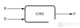
In addition to the control R and the index P , a perturbation acts in the systems. Perturbations are denoted as D = { d 1 , d 2 , ...}, see fig. 30.13. A disturbance is an input that, unlike the control parameter, does not depend on the will of the system owner. For example, low temperatures on the street, competition reduce, unfortunately, the flow of customers, equipment failure annoyingly reduce system performance. And the owner of the system cannot directly control these values. Typically, a disturbance acts "out of spite" to the owner, reducing the effect P of the control effort R. This is because, in general, the system is created to achieve goals that cannot be achieved by themselves in nature. By organizing a system, a person always hopes by means of it to attain some goal P. To this he spends the efforts of R , going against nature. A system is an organization of the natural components that are accessible to man, he has studied for achieving a certain new goal, previously unattainable in other ways.
| |
| Fig. 30.13. Symbol of the system under study, which are influenced by control actions R and disturbances D |
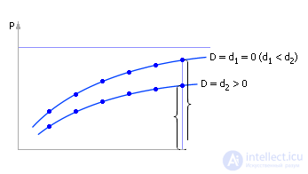
So, if we remove the dependence of the index P on the control R once more (as shown in Fig. 30.10), but under the conditions of the appeared perturbation D , then, perhaps, the nature of the curve will change. Most likely, the indicator will be lower for the same values of controls, since the disturbance is of a “nasty” character, reducing the performance of the system (see. Fig. 30.14). A system left to itself, without the efforts of a controlling character, ceases to provide the goal for which it was created . If, as before, to build the dependence of costs, correlate it with the dependence of the indicator on the control parameter, then the found extremum point will shift (see. Fig. 30.15) in comparison with the case of “disturbance = 0” (see. 30.12).
| |
| Fig. 30.14. Dependence of the indicator P on the control parameter R at various values of disturbances acting on the system D |
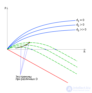
If the disturbance is increased again, the curves will change (see. Fig. 30.14) and, as a result, the position of the extremum point will change again (see. Fig. 30.15).
| |
| Fig. 30.15. Finding the extremum point on the total dependence at different values of the current perturbing factor D |
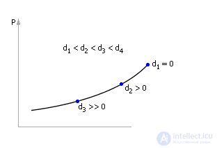
Ultimately, all the found positions of the extremum points are transferred to the new graph, where they form the dependence of the Indicator P on the Control parameter R as Perturbations D change (see. Fig. 30.16).
| |
| Fig. 30.16. The dependence of the indicator P from the manager parameter R when changing the values of perturbations D (the curve consists only of extremum points) |
Please note that in fact there are other working points on this graph (the graph is riddled with, as it were, families of curves), but the points plotted by us set such coordinates of the control parameter at which, given the disturbances (!), The greatest possible value of the indicator P is reached .
This graph (see Fig. 30.16) connects Indicator P , Management (resource) R and Perturbation D in complex systems, indicating how the decision maker (the decision maker) works best in the conditions of perturbations that have arisen. Now the user can, knowing the real situation on the object (the value of the perturbation), quickly determine by schedule what control action on the object is necessary to ensure the best value of the indicator of interest.
Note that if the control action is less than optimal, then the total effect will decrease, a situation of lost profit will arise. If the control action is more than optimal, the effect will also decrease, since it will be necessary to pay for the next increase in control efforts in magnitude greater than the one that you receive as a result of its use (bankruptcy situation).
Note In the text of the lecture, we used the words "management" and "resource", that is, we considered that R = U. It should be clarified that management really plays a role of some limited value for the owner of the system. That is, it is always a valuable resource for it, for which it is always necessary to pay, and which is always lacking. Indeed, if this value were not limited, then we could reach at the expense of the infinite size of the controls of infinitely large values of the targets, but the infinitely large results in nature are clearly not observed.
Sometimes, the actual management of U and the resource R are distinguished, calling the resource some reserve, that is, the limit of the possible value of the control action. In this case, the concepts of resource and control do not coincide: U < R . Sometimes, the limit value of the control U ≤ R and the integral resource ∫ U d t ≤ R are distinguished.


Comments
To leave a comment
System modeling
Terms: System modeling