Statistical modeling

Statistical modeling is a basic modeling method, consisting in the fact that a model is tested by a multitude of random signals with a given probability density. The goal is to statistically determine the output. The basis of statistical modeling is the Monte Carlo method . Recall that imitation is used when other methods cannot be applied.

Monte Carlo method

Consider the Monte Carlo method on the example of calculating the integral, the value of which cannot be found analytically.

Task 1. Find the value of the integral:

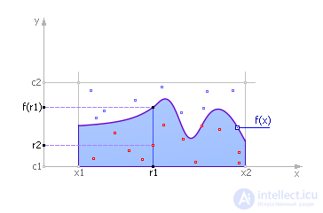
In fig. 21.1 is a graph of the function f ( x ). To calculate the value of the integral of this function is to find the area under this graph.

Fig. 21.1. Determining the value of the integral Monte Carlo method

We limit the curve at the top, right and left. Randomly distribute points in the search rectangle. Denote by N _{1 the} number of points taken for testing (that is, caught in a rectangle, these points are shown in Fig. 21.1 in red and blue), and N ₂ is the number of points under the curve, that is, in the filled area under the function (these the dots are shown in Fig. 21.1 in red). Then it is natural to assume that the number of points that fall under the curve with respect to the total number of points is proportional to the area under the curve (the integral value) with respect to the area of ​​the test rectangle. Mathematically, this can be expressed as:

These arguments, of course, are statistical, and all the more so, the greater the number of test points we take.

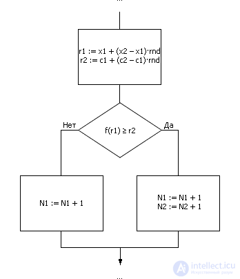
A fragment of the Monte Carlo algorithm in the form of a flowchart looks like it is shown in the picture. 21.2.

Fig. 21.2. Fragment of the implementation algorithm Monte Carlo method

The values ​​of r ₁ and r ₂ in fig. 21.2 are uniformly distributed random numbers from the intervals ( x ₁ ; x ₂ ) and ( c ₁ ; c ₂ ), respectively.

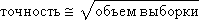
The Monte Carlo method is extremely efficient, simple, but a “good” random number generator is needed. The second problem of applying the method is to determine the sample size, that is, the number of points needed to provide a solution with a given accuracy. Experiments show that in order to increase the accuracy by 10 times, the sample size must be increased 100 times; that is, the accuracy is roughly proportional to the square root of the sample size:

The scheme of using the Monte Carlo method in the study
systems with random parameters

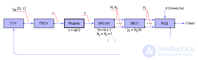
Having built a model of a system with random parameters, input signals from a random number generator (RNG) are sent to its input, as shown in fig. 21.3. RNG is designed so that it gives uniformly distributed random numbers r _pp from the interval [0; one]. Since some events may be more likely, others less likely, uniformly distributed random numbers from the generator feed the converter of the law of random numbers (CRL), which converts them into a user- defined law of probability distribution, for example, a normal or exponential law. These converted random numbers x are input to the model. The model fulfills the input signal x according to some law y = φ ( x ) and receives the output signal y , which is also random.

Fig. 21.3. General scheme of the method of statistical modeling

Filters and counters are installed in the statistics accumulation unit (BNStat). The filter (some logical condition) determines, by the value of y , whether a particular event was realized in a particular experiment (condition fulfilled, f = 1) or not (condition not fulfilled, f = 0). If the event has been realized, the event counter is incremented by one. If the event did not materialize, the counter value does not change. If you want to keep track of several different types of events, then for statistical modeling you will need several filters and counters N _i . Always count the number of experiments - N.

Further, the ratio of N _i to N , calculated in the block for calculating statistical characteristics (BVSH) by the Monte Carlo method, gives an estimate of the probability p _{i of} occurrence of event i , that is, indicates the frequency of its loss in a series of N experiments. This allows to draw conclusions about the statistical properties of the simulated object.

For example, event A occurred as a result of 200 experiments conducted 50 times. This means, according to the Monte Carlo method, that the probability of making an event is: p _A = 50/200 = 0.25. The probability that an event does not occur is, respectively, 1 - 0.25 = 0.75.

Pay attention: when they talk about the probability obtained experimentally, it is called a frequency; the word probability is used when they want to emphasize that we are talking about a theoretical concept.

With a large number of experiments N, the frequency of occurrence of an event, obtained experimentally, tends to the value of the theoretical probability of an event occurring.

In the block of reliability assessment (AML), the degree of reliability of statistical experimental data taken from the model is analyzed (taking into account the accuracy of the result ε given by the user) and the number of statistical tests required for this is determined. If the fluctuation of the frequency of occurrence of events relative to the theoretical probability is less than the specified accuracy, then the experimental frequency is accepted as an answer, otherwise the generation of random input actions is continued, and the simulation process is repeated. With a small number of tests, the result may be unreliable. But the more trials, the more accurate the answer, according to the central limit theorem.

Note that the evaluation is carried out at the worst of frequencies. This provides a reliable result at once on all the removed characteristics of the model.

Example 1. We solve a simple problem. What is the probability of a coin falling out by an eagle up when it is randomly dropped from a height?

Let's start toss a coin and record the results of each throw (see table. 21.1).

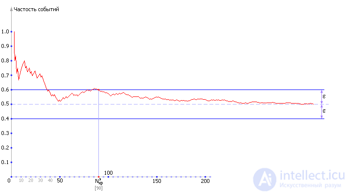
We will calculate the frequency of the eagle's fallout as the ratio of the number of cases of the eagle's fallout to the total number of observations. Look at table. 21.1. cases for N = 1, N = 2, N = 3 — first, the values ​​of the frequency cannot be called reliable. Let us try to plot the dependence of P _о on N - and see how the frequency of the eagle's loss varies depending on the number of experiments performed. Of course, with different experiments different tables will be obtained and, therefore, different graphs. In fig. 21.4 shows one of the options.

Fig. 21.4. Experimental dependence of the frequency of occurrence of a random event on the number of observations and its desire for a theoretical probability

We draw some conclusions.

1. It can be seen that for small values ​​of N , for example, N = 1, N = 2, N = 3, the answer cannot be trusted at all. For example, P _о = 0 with N = 1, that is, the probability of a falling eagle with one throw is zero! Although everyone is well aware that this is not the case. That is, until we received a very rude answer. However, look at the graph: in the process of accumulating information, the answer slowly but surely approaches the correct one (it is highlighted by a dotted line). Fortunately, in this particular case, we know the correct answer: ideally, the probability of an eagle falling out is 0.5 (in other, more complex tasks, the answer to us, of course, will be unknown). Suppose that we need to know the answer with an accuracy of ε = 0.1. Let us draw two parallel lines separated from the correct answer 0.5 at a distance of 0.1 (see. Fig. 21.4). The width of the corridor formed will be equal to 0.2. As soon as the P _o ( N ) curve enters this corridor so that it never leaves it, you can stop and see for what value of N this happened. This is the experimentally calculated critical value of the required number of experiments _Ncr to determine the answer with an accuracy of ε = 0.1; The ε- neighborhood in our reasoning plays the role of a kind of precision tube. Note that the answers P _о (91), P _о (92) and so on do not change their values ​​much (see Fig. 21.4); at least, they do not change the first digit after the comma, which we must trust in the conditions of the problem.
2. The reason for this behavior of the curve is the action of the central limit theorem (see lecture 25 and lecture 34). So far here we will formulate it in the simplest variant “The sum of random variables is a non-random quantity”. We used the average value of P _o , which carries information about the sum of the experiments, and therefore gradually this value becomes more and more reliable.
3. If we repeat this experience again, then, of course, its result will be a different kind of random curve. And the answer will be different, although about the same. We will conduct a series of such experiments (see fig. 21.5). Such a series is called an implementation ensemble. So what answer should you believe in the end? After all, even though they are close, they still differ. In practice, come in different ways. The first option is to calculate the average value of responses for several implementations (see Table 21.2).

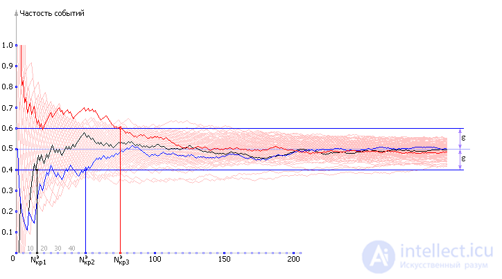
Fig. 21.5. Experimentally filmed random dependency ensemble the frequency of occurrence of a random event by the number of observations

We set up several experiments and determined each time how many experiments had to be done, that is, _Ncr . It was done 10 experiments, the results of which were summarized in Table. 21.2. According to the results of 10 experiments, the average value of _Ncr was calculated.

Thus, after conducting 10 implementations of different lengths, we determined that on average it was enough to make 1 implementation of a length of 94 coin tosses.

Another important fact. Look carefully at the graph in fig. 21.5. It draws 100 implementations - 100 red lines. Mark on it the abscissa N = 94 with a vertical bar. There is a percentage of red lines that did not have time to cross the ε- neighborhood, that is ( P ^exp - ε ≤ P ^theory ≤ P ^exp + ε ), and enter the accuracy corridor until N = 94. Pay attention to such lines 5 This means that 95 out of 100, that is, 95% of the lines, are reliably included in the indicated interval.

Thus, having carried out 100 implementations, we achieved approximately 95% confidence in the experimentally obtained probability of falling out of an eagle, determining it with an accuracy of 0.1. To compare the obtained result, we calculate the theoretical value of _Ncr theoretically. However, this will require introducing the concept of confidence probability Q _F , which shows how willing we are to believe the answer. For example, if Q _F = 0.95, we are ready to believe the answer in 95% of 100 cases. The formula for theoretical calculation of the number of experiments, which will be studied in detail in lecture 34, is: N _cr ^t = k ( Q _F ) · p · (1 - p ) / ε ² , where k ( Q _F ) is the Laplace coefficient, p is the probability of the eagle falling, ε is the accuracy (confidence interval). In tab. 21.3 the values ​​of the theoretical quantity of the number of necessary experiments for different Q _F are shown (for accuracy ε = 0.1 and probability p = 0.5).

As you can see, our estimate of the length of the implementation, equal to 94 experiments, is very close to the theoretical, equal to 96. Some discrepancy is due to the fact that, apparently, 10 realizations are not enough to accurately calculate N _cr ^e . If you decide that you need a result that you need to trust more, then change the value of the confidence probability. For example, the theory tells us that if the experiments will be 167, then only 1-2 lines from the ensemble will not enter the proposed tube of accuracy. But keep in mind, the number of experiments with increasing accuracy and reliability grows very quickly.

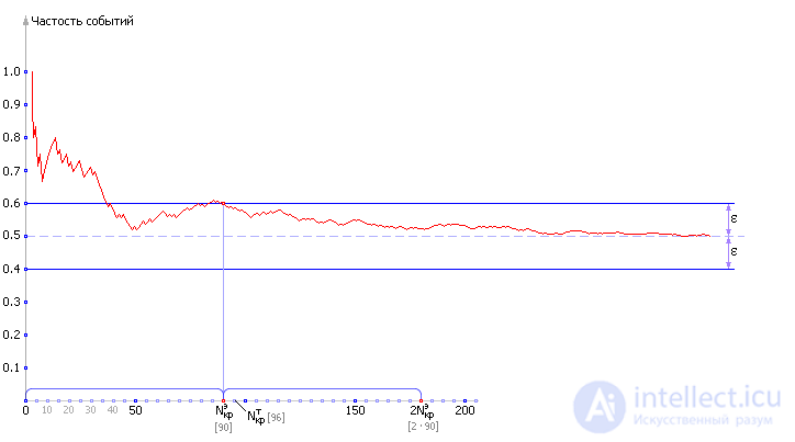
The second option used in practice is to carry out one implementation and increase the N _cr ^e obtained for it by 2 times . This is considered a good guarantee of the accuracy of the answer (see fig. 21.6).

Fig. 21.6. Illustration of the experimental definition of Ncr by the rule “multiply by two”

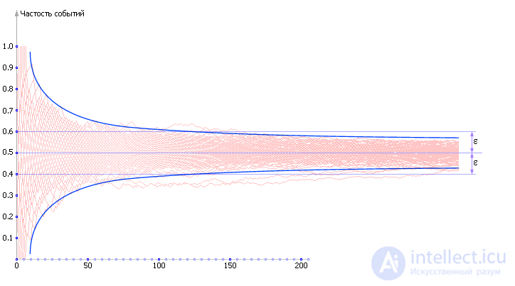
If you look at the ensemble of random realizations , you can find that the convergence of the particular to the value of theoretical probability occurs along a curve corresponding to the inverse quadratic dependence on the number of experiments (see Fig. 21.7).

Fig. 21.7. Illustration of the rate of convergence of the experimentally obtained frequency to theoretical probability

This is indeed what happens theoretically. If we change the given accuracy ε and investigate the number of experiments required to provide each of them, then we obtain a table. 21.4.

Construct a table. 21.4 graph of the dependence of N _cr ^t ( ε ) (see. Fig. 21.8).

Fig. 21.8. Dependence of the number of experiments required to achieve given accuracy ε with fixed Q F = 0.95

So, the considered graphs confirm the above assessment:

Note that there may be several accuracy estimates. Some of these will be discussed further in the presentation 34.

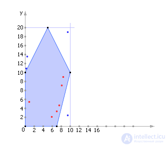
Example 2. Finding the area of ​​the figure by the Monte Carlo method. Determine the area of ​​the pentagon with the coordinates of the angles (0, 0), (0, 10), (5, 20), (10, 10), (7, 0) using the Monte Carlo method.

Draw a given pentagon in two-dimensional coordinates, inscribing it in a rectangle, whose area, as you might guess, is (10 - 0) · (20 - 0) = 200 (see. Fig. 21.9).

Fig. 21.9. Illustration to solve the problem about the area of ​​the figure by the Monte Carlo method

We use a table of random numbers to generate pairs of numbers R , G uniformly distributed in the interval from 0 to 1. The number R will simulate the coordinate X (0 ≤ X ≤ 10), therefore, X = 10 · R. The number G will imitate the Y coordinate (0 ≤ Y ≤ 20), therefore, Y = 20 · G. Generate 10 numbers of R and G and display 10 points ( X ; Y ) in Fig. 21.9 and in table. 21.5.

The statistical hypothesis is that the number of points in the outline of the figure is proportional to the area of ​​the figure: 6:10 = S : 200. That is, according to the formula of the Monte Carlo method, we obtain that the area S of the pentagon is: 200 · 6/10 = 120.

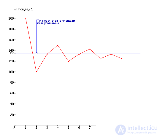
Let us see how the value of S has changed from experience to experience (see Table 21.6).

Since the answer still changes the value of the second digit, the possible inaccuracy is still more than 10%. The accuracy of the calculation can be increased with an increase in the number of tests (see fig. 21.10).

Fig. 21.10. Illustration of the process of convergence defined experimentally response to a theoretical result