Lecture
A mathematical model is a mathematical representation of reality , one of the variants of a model, as a system, the study of which allows to obtain information about some other system.
The process of building and studying mathematical models is called mathematical modeling .
All natural and social sciences that use the mathematical apparatus, in fact, are engaged in mathematical modeling: they replace the object of study with its mathematical model and then study the latter. The connection of the mathematical model with reality is carried out with the help of a chain of hypotheses, idealizations and simplifications. With the help of mathematical methods, an ideal object is described, as a rule, built on the stage of meaningful modeling .
No definition can fully cover the real-life activity in mathematical modeling. Despite this, definitions are useful in that they attempt to highlight the most significant features.
According to Lyapunov, mathematical modeling is an indirect practical or theoretical study of an object, in which it is not the object itself that interests us that is directly studied, but some auxiliary artificial or natural system (model) that is in some objective correspondence with a cognizable object and can replace it in certain respects and, in the course of its study, which gives information about the object itself being simulated .
In other variants, a mathematical model is defined as an object-substitute object of the original, providing the study of some properties of the original , as equivalent "of an object, reflecting in a mathematical form its most important properties - the laws to which it obeys, the connections inherent in its constituents parts " as a system of equations or arithmetic ratios, or geometrical shapes or a combination of both, the study of mathematics which means must answer these questions about the properties of a cos kupnosti real world object properties as a set of mathematical relations, equations inequalities describing basic patterns inherent studied process, object or system
The formal classification of models is based on the classification of mathematical tools used. Often built in the form of dichotomies. For example, one of the popular dichotomy sets :
and so on. Each constructed model is linear or nonlinear, deterministic or stochastic, ... Naturally, mixed types are possible: concentrated in one respect (in terms of parameters), distributed models in the other, and so on.
Along with the formal classification, the models differ in the way the object is represented:
Structural models represent an object as a system with its own device and functioning mechanism. Functional models do not use such representations and reflect only the externally perceived behavior (functioning) of the object. In their limiting terms, they are also called “black box” models. Combined model types are also possible, sometimes referred to as gray box models.
Practically all authors describing the process of mathematical modeling indicate that a special ideal construction is first built, a meaningful model . There is no settled terminology here, and other authors call this ideal object a conceptual model , a speculative model or a premodel . In this case, the final mathematical construction is called the formal model or simply the mathematical model obtained as a result of the formalization of this content model (pre-model). Building a meaningful model can be done using a set of ready-made idealizations, as in mechanics, where ideal springs, solids, ideal pendulums, elastic media, etc., provide ready-made structural elements for meaningful modeling. However, in areas of knowledge where there are no fully completed formalized theories (the leading edge of physics, biology, economics, sociology, psychology, and most other areas), the creation of meaningful models is greatly complicated.
Peierls provided a classification of mathematical models used in physics and, more broadly, in the natural sciences. In the book of A.N. Gorban and R. G. Khlebopros [17], this classification was analyzed and expanded. This classification is focused, first of all, on the stage of building the content model.
Models of the first type are hypotheses ( “this could be” ), “represent a tentative description of a phenomenon, and the author either believes in its possibility, or even considers it to be true.” According to Peierls, this is, for example, the Ptolemy model of the Solar System and the Copernican model (improved by Kepler), the Rutherford atom model and the Big Bang model.
Hypothesis models in science cannot be proved once and for all; one can only talk about their refutation or non-refusal as a result of an experiment [18] .
If a model of the first type is built, this means that it is temporarily recognized as true and you can concentrate on other problems. However, this cannot be a point in research, but only a temporary pause: the status of a model of the first type can only be temporary.
The second type - the phenomenological model ( “we behave as if ...” ) contains a mechanism for describing the phenomenon, although this mechanism is not sufficiently convincing, cannot be sufficiently confirmed by the available data or does not agree well with the existing theories and accumulated knowledge about the object. Therefore, phenomenological models have the status of temporary solutions. It is believed that the answer is still unknown, and it is necessary to continue the search for "true mechanisms." For the second type, Peierls includes, for example, models of caloric and quark models of elementary particles.
The role of the model in the study may change over time, it may happen that new data and theories will confirm the phenomenological models and those will be upgraded to the status of a hypothesis. Similarly, new knowledge can gradually come into conflict with hypothetical models of the first type, and those can be transferred to the second. Thus, the quark model gradually goes into the category of hypotheses; atomism in physics arose as a temporary solution, but with the course of history it moved to the first type. But the ether models have made their way from type 1 to type 2, and now they are outside of science.
The idea of simplification is very popular when building models. But the simplification is different. Peierls identifies three types of simplifications in modeling.
The third type of model is approximation ( “we consider something very large or very small” ). If it is possible to construct equations describing the system under study, this does not mean that they can be solved even with the help of a computer. A common technique in this case is the use of approximations (type 3 models). Among them are linear response models . Equations are replaced by linear ones. The standard example is Ohm’s law.
If we use the ideal gas model to describe sufficiently rarefied gases, then this is a type 3 model (approximation). At higher gas densities, it is also useful to imagine a simpler situation with an ideal gas for a qualitative understanding and assessment, but then this is type 4.
The fourth type is simplification ( “omitting certain details for clarity” ), details are thrown into this, which can noticeably and not always controlfully affect the result. The same equations can serve as a model of type 3 (approximation) or 4 (omitting certain details for clarity) - this depends on the phenomenon for which the model is used. So, if linear response models are applied in the absence of more complex models (that is, non-linear equations are not linearized, but linear equations describing the object are simply searched), then these are phenomenological linear models , and they refer to the following type 4 (all non-linear details for clarity "omit).
Examples: the application of the ideal gas model to a non-ideal gas, the van der Waals equation of state, most models of solid-state physics, liquids, and nuclear physics. The path from microdescription to the properties of bodies (or media) consisting of a large number of particles is very long. We have to throw many details. This leads to models of the fourth type.
The fifth type is a heuristic model ( “there is no quantitative confirmation, but the model contributes to a deeper insight into the essence of the matter” ), such a model retains only a qualitative similarity to reality and gives predictions only “in order of magnitude”. A typical example is the approximation of the mean free path in kinetic theory. It gives simple formulas for viscosity, diffusion, and thermal conductivities, consistent with reality in order of magnitude.
But when building a new physics, it is far from immediately obtained a model that gives at least a qualitative description of the object - a model of the fifth type. In this case, a model is often used by analogy , reflecting the reality at least in some features.
Type six is a model analogy ( “we will take into account only certain features” ). Peierls cites the history of using analogies in Heisenberg's first article on the nature of nuclear forces [19] .
The seventh type of models is a thought experiment ( “the main thing is to disprove the possibility” ). This type of modeling was often used by Einstein, in particular, one of these experiments led to the construction of a special special theory of relativity. Suppose that in classical physics we are moving behind a light wave at the speed of light. We will observe periodically varying in space and a constant in time electromagnetic field. According to Maxwell's equations, this can not be. From here, Einstein concluded: either the laws of nature change when the reference system changes, or the speed of light depends on the reference system, and chose the second option.
The eighth type is the demonstration of possibility ( “the main thing is to show the internal consistency of the possibility” ), such models are also mental experiments with imaginary entities, demonstrating that the intended phenomenon is consistent with the basic principles and is internally inconsistent. This is the main difference from models of type 7, which reveal hidden contradictions.
One of the most famous such experiments is Lobachevsky's geometry. (Lobachevsky called it “imaginary geometry.”) Another example is the mass production of formally kinetic models of chemical and biological wheels, autowaves. The Einstein-Podolsky-Rosen paradox was conceived as a thought experiment to demonstrate the inconsistency of quantum mechanics, but in an unplanned way with time turned into a model 8 of the type — a demonstration of the possibility of quantum teleportation of information.
The basis of the content classification is the stages preceding the mathematical analysis and calculations. The eight types of models by Peierls are eight types of research positions in modeling.
Consider a mechanical system consisting of a spring fixed at one end, and a load of mass  attached to the free end of the spring. We assume that the load can move only in the direction of the spring axis (for example, the movement occurs along the rod). Let's build a mathematical model of this system. We will describe the state of the system by distance
  from the center of the load to its equilibrium position. We describe the interaction of the spring and the load using Hooke's law (
  ), after which we use Newton's second law to express it in the form of a differential equation:
 ,
,
Where  means the second derivative of on time:
  .
.
The resulting equation describes a mathematical model of the considered physical system. This model is called the “harmonic oscillator”.
According to the formal classification, this model is linear, deterministic, dynamic, focused, continuous. In the process of its construction, we have made many assumptions (about the absence of external forces, the absence of friction, small deviations, etc.), which in reality may not be fulfilled.
In relation to reality, this is most often a type 4 model simplification (“omit some details for clarity”), since some essential universal features (for example, dissipation) are omitted. In a certain approximation (say, while the deviation of the load from equilibrium is small, with little friction, for not too much time, and under certain other conditions), this model describes the real mechanical system quite well, since the discarded factors have a negligible effect on its behavior. . However, the model can be refined by taking into account some of these factors. This will lead to a new model, with a wider (albeit again limited) area of applicability.
However, when refining the model, the complexity of its mathematical research can increase significantly and make the model virtually useless. Often, a simpler model allows for a better and deeper investigation of a real system than a more complex (and, formally, “more correct”).
If we apply the model of a harmonic oscillator to objects far from physics, its meaningful status may be different. For example, when this model is applied to biological populations, it should most likely be attributed to type 6 analogy (“we will take into account only some peculiarities”).
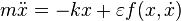
The harmonic oscillator is an example of the so-called “hard” model. It is obtained as a result of a strong idealization of the real physical system. The properties of a harmonic oscillator are qualitatively changed by small perturbations. For example, if you add a small term to the right side  (friction) (
  - some small parameter), then we obtain exponentially decaying *** collars if we change the sign of the additional term
  then the friction will turn into pumping and the amplitude of the stake *** will exponentially increase.
To solve the problem of the applicability of a rigid model, it is necessary to understand how significant are the factors that we have neglected. It is necessary to investigate soft models, which are obtained by a small perturbation of a rigid one. For a harmonic oscillator, they can be given, for example, by the following equation:
 .
.
Here  —A certain function in which the friction force or the dependence of the spring stiffness coefficient on the degree of its stretching can be taken into account. Explicit view of the function
  we are not interested at the moment.
If we prove that the behavior of the soft model is not fundamentally different from the behavior of a rigid one (regardless of the explicit type of perturbing factors, if they are small enough), the task will be reduced to the study of a rigid model. Otherwise, the application of the results obtained in the study of a rigid model will require additional research.
If the system retains its qualitative behavior with a small perturbation, it is said that it is structurally stable. The harmonic oscillator is an example of a structurally unstable (non-coarse) system. [20] However, this model can be used to study processes for limited periods of time.
The most important mathematical models usually have an important property of universality : fundamentally different real phenomena can be described by the same mathematical model. Скажем, гармонический осциллятор описывает не только поведение груза на пружине, но и другие коле***тельные процессы, зачастую имеющие совершенно иную природу: малые коле***ния маятника, коле***ния уровня жидкости в  -образном сосуде или изменение силы тока в коле***тельном контуре. Таким образом, изучая одну математическую модель, мы изучаем сразу целый класс описываемых ею явлений. Именно этот изоморфизм законов, выражаемых математическими моделями в различных сегментах научного знания, подвиг Людвига фон Берталанфи на создание «общей теории систем».
Существует множество задач, связанных с математическим моделированием. Во-первых, надо придумать основную схему моделируемого объекта, воспроизвести его в рамках идеализаций данной науки. Так, вагон поезда превращается в систему пластин и более сложных тел из разных материалов, каждый материал задается как его стандартная механическая идеализация (плотность, модули упругости, стандартные прочностные характеристики), после чего составляются уравнения, по дороге какие-то детали отбрасываются как несущественные, производятся расчёты, сравниваются с измерениями, модель уточняется, и так далее. Однако для разработки технологий математического моделирования полезно разобрать этот процесс на основные составные элементы.
Традиционно выделяют два основных класса задач, связанных с математическими моделями: прямые и обратные.
Прямая задача : структура модели и все её параметры считаются известными, главная задача — провести исследование модели для извлечения полезного знания об объекте. Какую статическую нагрузку выдержит мост? Как он будет реагировать на динамическую нагрузку (например, на марш роты солдат, или на прохождение поезда на различной скорости), как самолёт преодолеет звуковой барьер, не развалится ли он от флаттера, — вот типичные примеры прямой задачи. Постановка правильной прямой задачи (задание правильного вопроса) требует специального мастерства. Если не заданы правильные вопросы, то мост может обрушиться, даже если была построена хорошая модель для его поведения. Так, в 1879 г. в Великобритании обрушился металлический железнодорожный мост через реку Тей [en] , конструкторы которого построили модель моста, рассчитали его на 20-кратный запас прочности на действие полезной нагрузки, но забыли о постоянно дующих в тех местах ветрах. И через полтора года он рухнул. [21]
В простейшем случае (одно уравнение осциллятора, например) прямая задача очень проста и сводится к явному решению этого уравнения.
Обратная задача : известно множество возможных моделей, надо выбрать конкретную модель на основании дополнительных данных об объекте. Чаще всего структура модели известна, и необходимо определить некоторые неизвестные параметры. Дополнительная информация может состоять в дополнительных эмпирических данных, или в требованиях к объекту ( задача проектирования ). Дополнительные данные могут поступать независимо от процесса решения обратной задачи ( пассивное наблюдение ) или быть результатом специально планируемого в ходе решения эксперимента ( активное наблюдение ).
Одним из первых примеров виртуозного решения обратной задачи с максимально полным использованием доступных данных был построенный Ньютоном метод восстановления сил трения по наблюдаемым затухающим коле***ниям.
В качестве другого примера можно привести математическую статистику. Задача этой науки — разработка методов регистрации, описания и анализа данных наблюдений и экспериментов с целью построения вероятностных моделей массовых случайных явлений [22] . То есть множество возможных моделей ограничено вероятностными моделями. В конкретных задачах множество моделей ограничено сильнее.
Для поддержки математического моделирования разработаны системы компьютерной математики, например, Maple, Mathematica, Mathcad, MATLAB, VisSim и др. [23] Они позволяют создавать формальные и блочные модели как простых, так и сложных процессов и устройств и легко менять параметры моделей в ходе моделирования. Блочные модели представлены блоками (чаще всего графическими), набор и соединение которых задаются диаграммой модели.
Согласно модели, предложенной Мальтусом, скорость роста пропорциональна текущему размеру популяции, то есть описывается дифференциальным уравнением:
 ,
,
Where  — некоторый параметр, определяемый разностью между рождаемостью и смертностью. Решением этого уравнения является экспоненциальная функция
 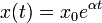 . Если рождаемость превосходит смертность (
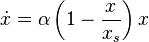
  ), размер популяции неограниченно и очень быстро возрастает. В действительности этого не может происходить из-за ограниченности ресурсов. При достижении некоторого критического объёма популяции модель перестает быть адекватной, поскольку не учитывает ограниченность ресурсов. Уточнением модели Мальтуса может служить логистическая модель, которая описывается дифференциальным уравнениемФерхюльста:
 ,
,
Where  — «равновесный» размер популяции, при котором рождаемость в точности компенсируется смертностью. Размер популяции в такой модели стремится к равновесному значению , причем такое поведение структурно устойчиво.
Допустим, что на некоторой территории обитают два вида животных: кролики (питающиеся растениями) и лисы (питающиеся кроликами). Пусть число кроликов , число лис  . Используя модель Мальтуса с необходимыми поправками, учитывающими поедание кроликов лисами, приходим к следующей системе, носящей имя модели Лотки — Вольтерры :
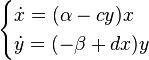
Эта система имеет равновесное состояние, когда число кроликов и лис постоянно. Отклонение от этого состояния приводит к колебаниям численности кроликов и лис, аналогичным колебаниям гармонического осциллятора. Как и в случае гармонического осциллятора, это поведение не является структурно устойчивым: малое изменение модели (например, учитывающее ограниченность ресурсов, необходимых кроликам) может привести к качественному изменению поведения. Например, равновесное состояние может стать устойчивым, и колебания численности будут затухать. Возможна и противоположная ситуация, когда любое малое отклонение от положения равновесия приведет к катастрофическим последствиям, вплоть до полного вымирания одного из видов. На вопрос о том, какой из этих сценариев реализуется, модель Вольтерры — Лотки ответа не дает: здесь требуются дополнительные исследования

Comments
To leave a comment
System modeling
Terms: System modeling