Lecture
The normal distribution law is found in nature quite often, so some effective modeling methods have been developed for it. The formula for the probability distribution of the values of a random variable x according to the normal law is:
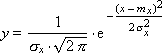
As can be seen, the normal distribution has two parameters: the expectation m x and the standard deviation σ x of x from this expectation.
|
A normalized normal distribution is a normal distribution for which m x = 0 and σ x = 1. From the normalized distribution, you can get any other normal distribution with given m x and σ x using the formula: z = m x + x · σ x .
Considering the last formula, remember computer graphics formulas: the scaling operation is expressed in a mathematical model through multiplication (this corresponds to a change in the magnitude spread, stretching a geometric image), the displacement operation is expressed through addition (this corresponds to a change in the value of the most probable value, displacement of the geometric image).
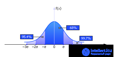
The normal distribution function is bell-shaped. In fig. 25.1 shows the normalized normal distribution.
|
|
| Fig. 25.1. Graphic view of normal law distribution of a random variable x with parameters m x = 0 and σ x = 1 (distribution is normalized) |
The graph in fig. 25.1 shows that in the region - σ < x < σ 68% of the distribution area is concentrated on the graph, in the area –2 σ < x <2 σ 95.4% of the distribution area is concentrated on the graph, in the area –3 σ < x <3 σ on the graph 99.7% of the distribution area is concentrated (the “three sigma rule”). Remember, please, rice. 2.7 from lecture 02.
Example. By normal distribution, the growth of people who are simultaneously in a large audience is distributed. Namely: quite a few people of very large height, and just as likely to meet people of very small stature. Basically, it is easier to meet people of medium height - and the likelihood of this is great.
For example, the average height of people is basically 170 cm, that is, m x = 170. It is also known that σ x = 20. In fig. 25.1 it is shown that the share of people with growth from 150 to 190 (170 - 20 <170 <170 + 20) is 68% in the society. The proportion of people from 130 cm to 210 cm (170 - 2 · 20 <170 <170 + 2 · 20) is 95.4% in the society. The proportion of people from 110 cm to 230 (170 - 3 · 20 <170 <170 + 3 · 20) is 99.7% in the society. For example, the probability that a person will be less than 110 cm tall or more than 230 cm is only 3 people per 1000.
A change in the normal distribution parameter m x leads to a shift of the curve along the x axis (see fig. 25.2).
|
|
| Fig. 25.2. The effect of the parameter "mathematical expectation" on the type of the law of the normal distribution of a random variable x |
A change in the parameter of the normal distribution σ x leads to scaling of the shape along the x axis (we recall, in any case, the area under the probability density curve is always the same and is equal to 1).
The more random the process, the smaller its standard deviation, the narrower and higher the bell on the graph. Changing the parameter of the normal distribution σ x leads to scaling the form (see fig. 25.3) along the x axis (we recall, in any case, the area under the probability density curve is always the same and equal to 1).
|
|
| Fig. 25.3. The effect of the “rms deviation "by the appearance of the law of normal distribution of random variable x |
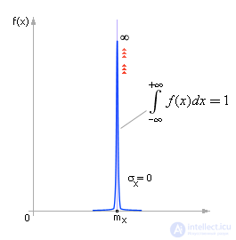
The more random the process, the smaller its standard deviation, the narrower and higher the bell on the graph. Indeed, the variation of randomness with respect to the expectation is becoming increasingly minimal. In the limit, the deterministic process has the form shown in fig. 25.4.
|
|
| Fig. 25.4. Type of law of normal probability distribution when passing to the deterministic case in the limit (σ x = 0). Random event becomes deterministic: x = m x ± 0 (no variation) |
Learning deterministic processes is easier. The greater the value of σ x , the less regular the behavior of the object being studied, since any values characterizing its parameters are possible, the spread of values relative to the average expected increases. Prediction and control of the behavior of the object in this case is difficult.
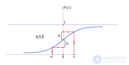
Consider the form of the integral density curve of the distribution of a random variable, distributed according to the normal law. Its view is shown in Fig. 25.5. F is the integral Laplace function. The meaning of the integral function is the probability that the random variable will take values from the range from –∞ to x . For example, the entry F (170) = 0.5 for our example means: the probability that a person randomly selected from the audience will not rise more than 170 cm is 0.5 (that is, every second).
|
|
| Fig. 25.5. View of the integral function of Laplace F (x) |
This function is given by the integral of the probability density of the normal distribution:

Unfortunately, this integral is not taken in the general form, therefore the Laplace function is given in the table for m x = 0 and σ x = 1. Since the Laplace function is symmetric about the point ( x = 0, y = 0.5) (like the function of the normal distribution ), F (- x ) = 1 - F ( x ), then the table contains only one of its symmetrical parts.
If the integration interval of the Laplace function is specified [ a ; b ], then:
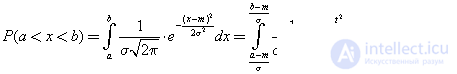
The probability of getting X in the interval, symmetric with respect to m x :

For example, for the “three sigma” rule: P (| x - m x | <3 σ ) = 2 · F (3) - 1 = 2 · 0.9987 - 1 = 0.9973 (as we indicated earlier). The number F (3) = 0.9987 is taken from the Laplace table.
Example. Find the probability of manufacturing a part with an error in its dimensions no more than 15 mm, if it is known that the manufacture of a part with an error is distributed according to the normal law m = 0 and σ = 10 mm.
P (| x | <15) = P (–15 < x <15) = F ((15 - 0) / 10) - F ((–15 - 0) / 10) = F (1.5) - F (- 1.5) = F (1.5) - (1 -
- F (1.5)) = 2 · F (1.5) - 1 = 2 · 0.9332 - 1 = 0.8664. That is, 8664 parts out of 10,000 will have an error in the size of no more than 15 mm.
An important property of the law is that the normal distribution is the limit for various types of distributions, which follows from the central limit theorem: “For a large number N of random variables X with any distribution law, their sum is a random number with a normal distribution law”.
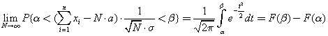
where a is the mathematical expectation in the distribution law of a random variable X ; σ is the standard deviation in the distribution law of the random variable X ; N is the number of random numbers.
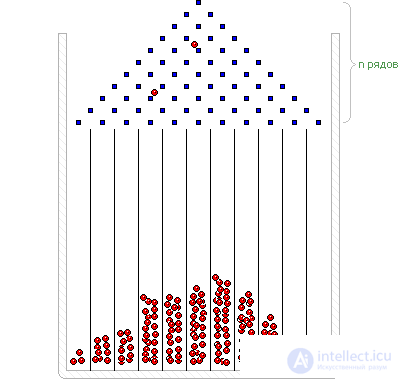
Recall the Galton Board experiment from physics (see Fig. 25.6).
|
|
| Fig. 25.6. Galton's board. Balls falling from above into a vessel by accident distributed in it in accordance with the normal distribution law |
The board is divided into sections; at the top of the board there are specially arranged rods, striking about which, a multitude of balls falling from above under the influence of gravity, also experiencing collisions between themselves, change their flight path. As a result, a different number of balls falls into different sections. If you wait for the end of the experience, then each section will have a certain number of balls, of course, each time is different, since the process of their collision is random. But it is interesting that the distribution of the balls into sections will form a normal distribution law. It seems that the board does not change, the balls fall the same, and nevertheless, firstly, the shape of the distribution fluctuates slightly (randomness), and different balls fall into different sections, secondly, at the macro level, where the organization of the balls aggregate, it always turns out the normal distribution law (pattern).
For an inquiring mind, experience raises very interesting questions. Why do small deviations in the behavior of system elements (balls) lead to large variations in their coordinates? Why are accidents not compensated? How much they are not compensated?
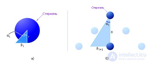
Denote by D the distance between the rods of the Galton board, r is the diameter of the rod (see Fig. 25.7, a, b). Obviously, the deviation of the β ball from the plumb trajectory at a small angle α (change of direction due to hitting the rod) can be calculated as tg ( α 1 ) = β 1 / r or α 1 ≈ β 1 / r (at small angles α 1 ). That is, then the ball flies at an angle α 1 to the free-fall trajectory at a distance D until it encounters a new rod. During the flight in a straight line from the rod to the rod, the ball will deviate from the vertical vertical line by the value β 2 = α 1 · D. Then again, having experienced a collision with rods, the ball will deviate by an angle α 2 ≈ β 2 / r and β 3 ≈ α 2 · D = β 1 · ( D / r ) 2 and so on.
|
|
| Fig. 25.7. The interaction of the balls with the rods of the board (detail) |
If the ball experiences n collisions, it will deviate from the steep trajectory by a distance of β n ≈ β 1 · ( D / r ) n - 1 (of course, if he is “lucky” and he will deviate all the time in one direction).
Now let's see how much this means in numbers, for example, D = 20 r , let the rods, from which the ball deviated in flight (collisions), n = 10, β 1 = 1 nm (distance less than an atom !!), then it is easy to calculate that β 10 = 10.24 km. That is, it can be seen that ultra-small deviations (1 nm and the number of collisions n = 10), in fact by chance, lead to macro effects. In fact, such a spread occurs much faster, since the balls also collide with each other. By the way, the removal of a ball for 10 km is also an incredible event, since the probability that the ball will be “lucky” 20 times in a row is an extremely unlikely number P = 0.520 = 10 - 6 .
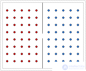
Consider another experiment, the Maxwell distribution. There are 40 blue and 40 red balls in the vessel, each in its own half of the vessel. The vessel halves are separated by a partition with a hole through which the balls can penetrate from one part of the vessel to another (see. Fig. 25.8). The number of balls, both blue and red, in each part of the vessel is counted.
|
|
| Fig. 25.8. The scheme of the experiment demonstrating diffusion (chaos) in complex systems |
The balls imitate the Brownian motion of molecules, colliding with each other elastically, exchanging energies, impulses, directions of velocity on impact, and also interacting with the walls of the vessel. With the elastic impact modeled in the experiment, the average kinetic energy of the particles encountered is averaged. Despite the fact that this is the essence of diffusion, that the balls were each color strictly in their half, over time approximately half (50%) of the red balls will be in the first half of the vessel, and half (50%) - in the second part of the vessel, the same also applies to blue balls (50%: 50%). The word “about” used here means that from time to time the totality of the balls will not be divided exactly into halves, but in proportion (50% ± h : 50% ± h ), since a random number of balls will pass from one part at random times vessel to another and vice versa. The relative fluctuation of average energies found in our experiments is rather large, of the order of 20%. Despite the fact that the balls of each color were strictly in their half (this is the essence of diffusion), over time, about half (50%) of the red balls will be in the first half of the vessel, and half (50%) - in the second part, the same applies to the blue balls (50%: 50%) (see fig. 25.9).
|
|
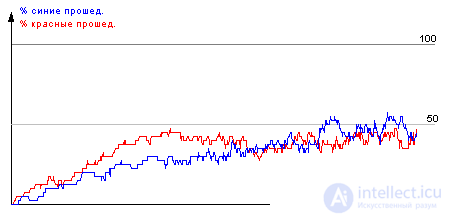
| Fig. 25.9. Typical behavior of characteristics in systems with diffusion. The figure shows the change in the number of blue and red molecules in one of the halves of the vessel with time |
Feature 1. You can continue to observe for as long as you wish, but at the same time the initial distribution of these balls will never be achieved. And, on the contrary, at any initial order of balls, the system will move to the same chaotic state. Why? The explanation for this is to be found in the fact that time is irreversible. The averaging operation is also irreversible. If I tell you that the sum of two numbers is equal to 8, then you can hardly say which ones I have chosen for this term. And many variants of the components lead to the same amount.
The chaotic system does not remember its past. Namely: over time, the state of such a system does not depend on how and from what state the system came to chaotic. From any initial state, our system rather quickly goes into this chaotic state, and is in it further for a long time. That is, the chaotic state is a steady state. It is interesting that in this steady state one can find such a number of parameters that will be unchanged with time, such parameters describe the system as a whole and are called macro parameters. For example, in our example, a stable macroparameter is the distribution of the number of molecules n modulo velocity v , which demonstrates Maxwell's law n ( v ) = r · v 2 · e - c · v 2 / T ( r , c are coefficients, T is the temperature of the population molecules).
Feature 2. If you divide a vessel into a larger number of parts, the balls will be distributed between them in approximately equal shares.
Peculiarity 3. The word "approximately" in half, tells us that in the answer 50%: 50% there is always a variation, dispersion, fluctuation. This spread decreases if the number of molecules in a vessel is increased.
Feature 4. If you start the model again and try to arrange the balls first, for example, set them in exactly rows in one half of the vessel, or at the top, or in one of the corners, then very quickly the balls "approximately" will be evenly distributed throughout the vessel, and chaos will occur, there is order will disappear and, interestingly, never come again. Where does chaos come from, how does the system move from order to chaos? The cause of chaos, as we have previously shown in the Galton Board experiment, appears at the moment of small deviations of the balls (for example, 10 –9 m) from the ideal theoretical trajectory, but this slight deviation of the distance D in flight leads to a significant deviation of the trajectory from ideal and collision of balls, which dramatically changes the trajectories of neighbors. Instantly, an avalanche of collisions appears, and chaos sets in very quickly.
Feature 5. Earlier, it was believed that systems with a small number of elements are not able to exhibit randomness, chaotic behavior. The reasoning of physicists about a gas of billions of molecules prevailed. Carry out the same experiment with five balls, then with three and, finally, with one ball. As a result of the experiment, the Maxwell distribution manifests itself rather stubbornly, however, this requires waiting a few times longer. (The exception will be the experience with one ball!) Experience shows that averaging over an ensemble of molecules and over time leads to the same result . So chaos can also occur on small sets.
So, both the Galton Board experience and the experimental removal of the Maxwell distribution lead us empirically to the fact that the normal distribution is widespread in the world around us. The summation of random variables, the sum of actions, the joint imposition of effects at the micro level often leads, by averaging, to the appearance of a normal distribution at the macro level.
Consider the issue of simulating random variables given by the normal distribution law.
For this, a normal number can be taken from the reference book in the table of the Laplace function and get a random number using the method of taking the inverse function (see Lecture 24): x = F –1 ( r ), where F is the integral Laplace function.
Technically, this means that it is necessary to play a random uniformly distributed number r from the interval [0; 1] with a standard RNG (see the table of absolutely random checked numbers), find an equal number in the table of values of the Laplace function in column F and determine the random variable x corresponding to this number from the line.
The disadvantage of the method is the need to store in the computer’s memory the entire table of the numbers of the Laplace function.
The general idea of the method is as follows: it is required to add random numbers with any distribution law, normalize them and convert them to the desired range of the normal distribution.
Suppose that for the purpose of imitation, we need to obtain a series of random numbers x distributed according to a normal law with given expectation m x and standard deviation σ x .

Example. Смоделировать поток заготовок для обработки их на станке. Известно, что длина заготовки колеблется случайным образом. Средняя длина заготовки составляет 35 см, а среднеквадратичное отклонение реальной длины от средней составляет 10 см. То есть по условиям задачи m x = 35, σ x = 10. Тогда значение случайной величины будет рассчитываться по формуле: V = r 1 + r 2 + r 3 + r 4 + r 5 + r 6 , где r — случайные числа из ГСЧ рр [0; 1], n = 6.
X = σ x · (sqrt(12/ n ) · ( V – n /2)) + m x = 10 · sqrt(2) · ( V – 3) + 35
or
X = 10 · sqrt(2) · (( r 1 + r 2 + r 3 + r 4 + r 5 + r 6 ) – 3) + 35.
Совсем простым методом получения нормальных чисел является метод Мюллера, использующий формулы: Z = √(–2 · Ln( r 1 )) · cos(2 π · r 2 ), где r 1 и r 2 — случайные числа из ГСЧ рр [0; one].
Можно также воспользоваться аналогичной формулой Z = √(–2 · Ln( r 1 )) · sin(2 π · r 2 ), где r 1 и r 2 — случайные числа из ГСЧ рр [0; one].
Example. Материал поступает в цех один раз в сутки по 10 штук сразу. Расход материала из цеха случайный по нормальному закону с математическим ожиданием m = 10 и среднеквадратичным отклонением σ = 3.5. Вычислить вероятность дефицита на складе при запасе материала в начальный момент времени 20 штук.
При реализации в среде моделирования Stratum решение задачи будет выглядеть следующим образом.
|
|


Comments
To leave a comment
System modeling
Terms: System modeling