Lecture
Kallman proved the theorem that any dynamic signal can be represented as:
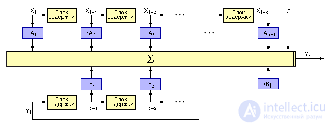
Y i = A 1 · X i + A 2 · X i - 1 + ... + B 1 · Y i - 1 + B 2 · Y i - 2 + ... + C.
| |
| Fig. 6.1. Graphic presentation Kallman filter on charts |
The idea of the Kallman filter is that the output of the system at the ith moment of time is determined by the input signal, its history and the history of the system state itself.
The more row members there are, that is, the more Y variables are taken into account in the model entry, the deeper the system's memory. Note that the presence of the term Y i - 1 in the model of a dynamic system corresponds to the presence of the first derivative, Y i - 2 - the second derivative, etc.
Suppose the following experimental data are known: the states of the signals X i and Y i at n time points (Table 6.1).
| Table 6.1. Table experimental data | ||||||||||||||||||
|
Since for each experimental point X i it is necessary to indicate its neighbors specified by a number, it is convenient to present the samples in the extended table used for the calculation (see Table 6.2).
| Table 6.2. Table of experimental data and intermediate calculations | |||||||||||||||||||||||||||||||||||
|
We find the error between the value of the experimentally taken point and its theoretical value (hypothesis):
E m = Y m - A 1 · X m - A 2 · X m - 1 - ... - B 1 · Y m - 1 - B 2 · Y m - 2 - ... - C.
The total error F (the sum is taken over all experimental points) should be minimized with respect to the defined variables A 1 , A 2 , ..., B 1 , B 2 , ..., C :
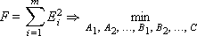
After taking the partial derivatives of F with respect to A 1 , A 2 , ..., B 1 , B 2 , ..., C , equating them to zero and creating a system of equations, we obtain a linear multiple regression model, from which the unknown coefficients A 1 , A 2 , ..., B 1 , B 2 , ..., C models.
Since the coefficients of the model are defined, we will construct an implementation (see Fig. 6.2) that simulates the behavior of the system described by the Callman filter.
| |
| Fig. 6.2. Variant of technical implementation of the Kallman filter |
The “delay unit” in the presented implementation is necessary in order to shift the signal to the clock and get the next sample for the next variable in the series of the model. Depending on the implementation environment, the delay block can be organized in different ways.
For example, in the case of the implementation of a delay unit in the Stratum-2000 modeling environment, the first method can be based on overwriting information from one variable (cell) to another, which requires one clock cycle. Thus, it is possible to arrange a signal delay for any number of cycles. For example, the delay of the signal X relative to Y will be 3 cycles if you perform the following sequence of operations: A1: = X; A2: = A1; Y: = A2.
In the second method, the delay is organized by means of an array: at each clock cycle it is necessary that the numbers be moved to neighboring cells.
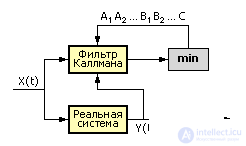
In fig. 6.3 shows the setup diagram (automatic finding coefficients).
| |
| Fig. 6.3. Automatic configuration scheme on-the-go model coefficients |
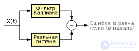
In fig. 6.4 is a diagram of checking the Kallman filter.
| |
| Fig. 6.4. Work Validation Scheme Callman filter models |


Comments
To leave a comment
System modeling
Terms: System modeling