Lecture
It is very convenient to describe the occurrence of random events in the form of probabilities of transitions from one state of the system to another, since it is considered that, going into one of the states, the system should not further take into account the circumstances of how it got into this state.
A random process is called a Markov process (or a process without aftereffect) if, for each time t, the probability of any state of the system in the future depends only on its state in the present and does not depend on how the system came to this state.
So, the Markov process is conveniently specified by the graph of transitions from state to state. We consider two options for describing Markov processes - with discrete and continuous time .
In the first case, the transition from one state to another occurs at a known point in time — ticks (1, 2, 3, 4, ...). The transition is carried out at each step, that is, the researcher is interested only in the sequence of states that the random process undergoes in its development, and does not care when exactly each transition occurs.
In the second case, the researcher is interested in both the chain of mutually changing states and the points in time at which such transitions occurred.
And further. If the transition probability does not depend on time, then a Markov chain is called homogeneous.
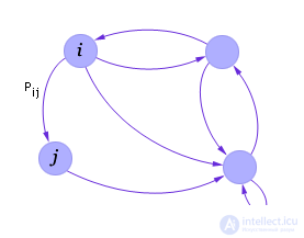
So, we represent the model of the Markov process as a graph in which the states (vertices) are interconnected by connections (transitions from the i -th state to the j -th state), see fig. 33.1.
| |
| Fig. 33.1. Transition graph example |
Each transition is characterized by a transition probability P ij . The probability P ij shows how often after hitting the i -th state, then the transition to the j -th state occurs. Of course, such transitions occur randomly, but if you measure the frequency of transitions for a sufficiently long time, it turns out that this frequency will coincide with a given transition probability.
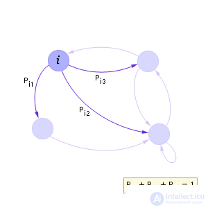
It is clear that for each state the sum of the probabilities of all transitions (outgoing arrows) from it to other states should always be equal to 1 (see Fig. 33.2).
| |
| Fig. 33.2. Transition Graph Fragment (transitions from the i-th state are full group of random events) |
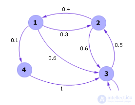
For example, the entire graph may look like the one shown in fig. 33.3.
| |
| Fig. 33.3. An example of a Markov transition graph |
The implementation of the Markov process (the process of its modeling) is the calculation of the sequence (chain) of transitions from state to state (see Fig. 33.4). The chain in fig. 33.4 is a random sequence and may also have other options for implementation.
| |
| Fig. 33.4. An example of a Markov chain modeled according to the Markov graph shown in fig. 33.3 |
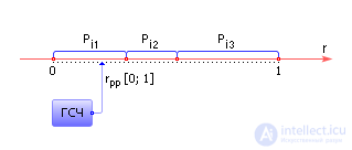
To determine which new state the process goes from the current i -th state, it suffices to split the interval [0; 1] for subintervals of P i 1 , P i 2 , P i 3 , ... ( P i 1 + P i 2 + P i 3 + ... = 1), see fig. 33.5. Next, using the RNG, it is necessary to obtain the next uniformly distributed in the interval [0; 1] random number r рр and determine which of the intervals it falls into (see Lecture 23).
| |
| Fig. 33.5. Process simulation of transition from i-th Markov chain states in the jth using random number generator |
After that, a transition to the state determined by the RNG is performed and the procedure described is repeated for the new state. The result of the model is a Markov chain (see. Fig. 33.4 ) .
Example. Imitation of firing a cannon at the target. In order to simulate shooting a cannon at a target, we will construct a model of a Markovian random process.
We define the following three states: S 0 - the target is not damaged; S 1 - the target is damaged; S 2 - the target is destroyed. Set the vector of initial probabilities:
|
The value of P 0 for each of the states shows what the probability of each of the states of the object is before firing.
Let's set the state transition matrix (see table. 33.1).
| Table 33.1. Transition Probability Matrix discrete Markov process | ||||||||||||||||||||
|
The matrix sets the probability of transition from each state to each. Note that the probabilities are set so that the sum of the transition probabilities from a certain state to the others is always equal to one (the system must go somewhere).
The model of the Markov process can be visualized as the following graph (see Fig. 33.6).
| |
| Fig. 33.6. Graph of the Markov process simulator shooting a gun on the target |
Using the model and method of statistical modeling, we will try to solve the following problem: to determine the average number of projectiles necessary for the complete destruction of the target.
We simulate, using a table of random numbers, the process of shooting. Let the initial state be S 0 . Take a sequence from a table of random numbers: 0.31, 0.53, 0.23, 0.42, 0.63, 0.21, ... (random numbers can be taken, for example, from this table).
0.31 : the target is in the S 0 state and remains in the S 0 state, since 0 < 0.31 <0.45;
0.53 : the target is in the S 0 state and transitions to the S 1 state, since 0.45 < 0.53 <0.45 + 0.40;
0.23 : the target is in the S 1 state and remains in the S 1 state, since 0 < 0.23 <0.45;
0.42 : the target is in the S 1 state and remains in the S 1 state, since 0 < 0.42 <0.45;
0.63 : the target is in the S 1 state and transitions to the S 2 state, since 0.45 < 0.63 <0.45 + 0.55.
Since the state S 2 is reached (the target goes from S 2 to S 2 with probability 1), the target is hit. To do this, in this experiment, it took 5 shells.
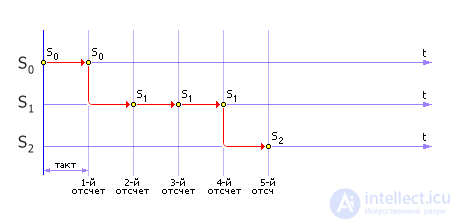
In fig. 33.7 shows the timing diagram, which is obtained during the described modeling process. The diagram shows how the process of state change occurs over time. The simulation cycle for this case has a fixed value. The very fact of the transition (what state the system goes to) is important for us and it doesn't matter when it happens.
| |
| Fig. 33.7. Timing Transition Chart Markov graph (an example of imitation) |
The target destruction procedure was completed in 5 cycles, that is, the Markov chain of this implementation looks as follows: S 0 - S 0 - S 1 - S 1 - S 1 - S 2 . Of course, this number cannot be the answer of the problem, since different implementations will produce different answers. And the answer to the problem can be only one.
Repeating this simulation, you can get, for example, even such implementations (it depends on what specific random numbers fall out): 4 ( S 0 - S 0 - S 1 - S 1 - S 2 ); 11 ( S 0 - S 0 - S 0 - S 0 - S 0 - S 1 - S 1 - S 1 - S 1 - S 1 - S 1 - S 2 ); 5 ( S 1 - S 1 - S 1 - S 1 - S 1 - S 2 ); 6 ( S 0 - S 0 - S 1 - S 1 - S 1 - S 1 - S 2 ); 4 ( S 1 - S 1 - S 1 - S 1 - S 2 ); 6 ( S 0 - S 0 - S 1 - S 1 - S 1 - S 1 - S 2 ); 5 ( S 0 - S 0 - S 1 - S 1 - S 1 - S 2 ). Total destroyed 8 targets. The average number of cycles in the firing procedure was: (5 + 4 + 11 + 5 + 6 + 4 + 6 + 5) / 8 = 5.75, or, rounding, 6. These are the shells, on average, it is recommended to have in stock a gun for destruction targets with such hit probabilities.
Now it is necessary to determine the accuracy. Precisely this can show us how much this answer should be trusted. To do this, let us see how the sequence of random (approximate) answers converges to the correct (exact) result. Recall that, according to the central limit theorem (see Lecture 25, Lecture 21), the sum of random variables is non-random, therefore, to obtain a statistically reliable answer, it is necessary to monitor the average number of projectiles obtained in a number of random realizations.
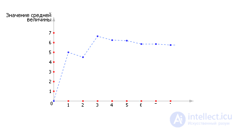
At the first stage of calculations, the average response was 5 rounds, at the second stage, the average response was (5 + 4) / 2 = 4.5 rounds, at the third - (5 + 4 + 11) / 3 = 6.7. Further, a series of averages, as statistics accumulate, looks like this: 6.3, 6.2, 5.8, 5.9, 5.8. If you depict this series as a graph of the average size of the projectiles released to hit a target, depending on the number of the experiment, you will find that this series converges to a certain value, which is the answer (see Fig. 33.8).
| |
| Fig. 33.8. The change in the average value depending on the number of the experiment |
Visually, we can observe that the graph “calms down”, the spread between the calculated current value and its theoretical value decreases with time, tending to a statistically accurate result. That is, at some point the graph enters into a certain “tube”, the size of which determines the accuracy of the answer.
The simulation algorithm will have the following form (see fig. 33.9).
Once again, we note that in the above case we do not care at which points in time the transition will occur. Transitions go tact by tact. If it is important to specify at what point in time the transition will occur, how long the system will stay in each of the states, you need to apply a model with continuous time.
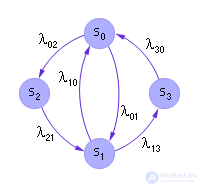
So, again, we represent the model of the Markov process in the form of a graph in which the states (vertices) are interconnected by connections (transitions from the i -th state to the j -th state), see fig. 33.10.
| |
| Fig. 33.10. Markov graph example process with continuous time |
Now each transition is characterized by a transition density λ ij . By definition:
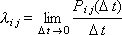
The density is understood as the probability distribution over time.
The transition from the ith state to the jth state occurs at random points in time, which are determined by the intensity of the transition λ ij .
The transition intensity (here, this concept coincides in meaning with the probability density distribution over time t ) is transferred when the process is continuous, that is, distributed in time.
With the flow intensity (and transitions are a flow of events) we have already learned how to operate lectures 28. Knowing the intensity λ ij of the occurrence of events generated by a flow, we can simulate a random interval between two events in this flow.

where τ ij - the time interval between the presence of the system in the i- th and j- th state.
Further, obviously, the system from any i -th state can go to one of several states j , j + 1, j + 2, ..., connected with it by the transitions λ ij , λ ij + 1 , λ ij + 2 , ....
In the jth state, it will go through τ ij ; in the ( j + 1) -th state, it will go through τ ij + 1 ; in the ( j + 2) -th state it goes through τ ij + 2 , etc.
It is clear that the system can go from the i -th state only to one of these states, and to that, the transition to which will occur earlier.
Therefore, from the sequence of times: τ ij , τ ij + 1 , τ ij + 2, and so on, you must select the minimum and determine the index j , indicating exactly which state the transition will take.
Example. Simulation of the machine. We will model the work of the machine (see. Fig. 33.10), which can be in the following states: S 0 - the machine is in good condition, free (idle); S 1 - the machine is serviceable, busy (processing); S 2 - the machine is serviceable, tool replacement (changeover) λ 02 < λ 21 ; S 3 - machine is faulty, repair is underway λ 13 < λ 30 .
Let us set the values of the parameters λ , using the experimental data obtained under production conditions: λ 01 - the flow for processing (without changeover); λ 10 - service flow; λ 13 - equipment failure rate; λ 30 - the flow of recovery.
The implementation will have the following form (see fig. 33.11).
| |
| Fig. 33.11. Sample simulation continuous Markov process with visualization on temporary chart (yellow color indicates prohibited, blue - realized states) |
In particular, from fig. 33.11 it can be seen that the implemented chain looks like this: S 0 - S 1 - S 0 - ... Transitions occurred at the following times: T 0 - T 1 - T 2 - T 3 - ..., where T 0 = 0, T 1 = τ 01 , T 2 = τ 01 + τ 10 .
Task. Since the model is being built in order to solve a problem on it, the answer to which until then was not at all obvious to us (see lecture 01), then we formulate such a problem for this example. Determine the proportion of time during the day, which takes a simple machine (count on the figure) T cf = ( T + T + T + T ) / N.
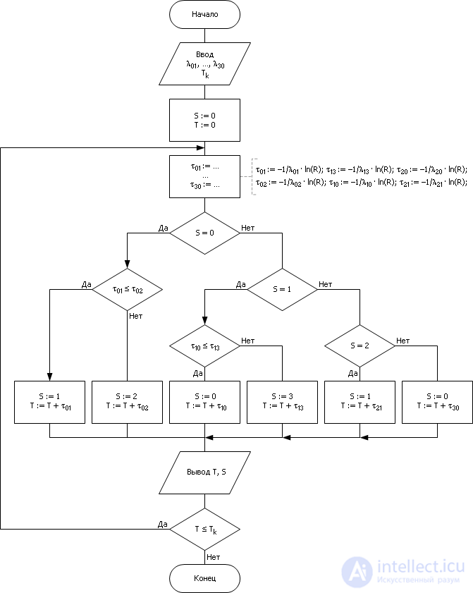
The simulation algorithm will have the following form (see. Fig. 33.12).
| |
| Fig. 33.12. A flowchart of a continuous simulation algorithm Markov process on the example of imitation of the machine |
Very often, the apparatus of Markov processes is used in the simulation of computer games, actions of computer heroes.


Comments
To leave a comment
System modeling
Terms: System modeling