Dynamic regression models defined as a transfer function

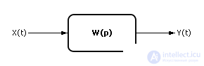
Let's build a regression model of a dynamic system using an example. Let's set the model in the form of transfer function (see fig. 5.1).

Fig. 5.1. Black box model in the form of transfer function

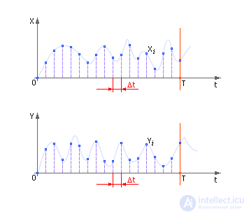
An exemplary view of the dynamic signals at the input and output is shown in Fig. 5.2. We confine ourselves to the time of consideration of signals equal to T.

Fig. 5.2. Possible type of dependence of the input signal X on time t and the dependence of the output signal Y on t for the case with continuous time

After sampling, associated with the processing of information on digital machines, these signals will look like shown in Fig. 5.3. Please note that the individual samples are separated from each other at a distance Δ t . It is important that the counts are often enough. The total of these samples is n , that is, T = n · Δ t ,

Fig. 5.3. Possible type of dependence of the input signal X on time t and the dependence of the output signal Y on t for the case of discrete time

Suppose that the dependencies shown in Fig. 5.2 and fig. 5.3, describes the transfer function of the following type (note that, as in lecture 02, the type of dependence is put forward hypothetically and the hypothesis must be, finally, confirmed or refuted):

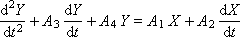
Replacing the “ p ” icon with “ d / dt ” (we draw your attention that such a replacement can be made only for the case of zero initial conditions: X (0) = 0 and Y (0) = 0) and considering that the transfer function is By definition, the ratio of the output to the input, that is, W = Y / X , we obtain the differential equation of the 2nd order:

We will integrate this expression twice and get for some arbitrary time t :

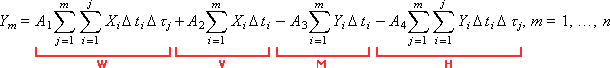
The coefficients A ₁ , A ₂ , A ₃ , A _{4 are} required to determine. To do this, we express the equation in a differential form in terms of the sums:

where n is the number of experimental points. Note that we have replaced the integrals and the continuous flow of time with sums and a discrete representation of time. To calculate the sums and double sums of experimentally defined dependences x and y , we use for convenience the table. 5.1 (in order not to overly clutter the table, we did not write in the sums Δ t _i and Δ τ _j ).

Table 5.1. Table of source data and auxiliary calculations

i X i Y i one X 1 Y 1 X 1 Y 1 X 1 Y 1 2 X 2 Y 2 X 1 + X 2 Y 1 + Y 2 2 X 1 + X 2 2 Y 1 + Y 2 3 X 3 Y 3 X 1 + X 2 + X 3 Y 1 + Y 2 + Y 3 3 X 1 + 2 X 2 + X 3 3 Y 1 + 2 Y 2 + Y 3 ... ... ... ... ... ... ... m X m Y m X 1 + X 2 + ... + X m Y 1 + Y 2 + ... + Y m m X 1 + ... + X m m Y 1 + ... + Y m ... ... ... ... ... ... ... n X n Y n X 1 + X 2 + ... + X n Y 1 + Y 2 + ... + Y n n X 1 + ... + X n n Y 1 + ... + Y n

The error at some m- th point can be written as:

As before, the error shows how much the theoretical value of Y _m deviates from the experimental value.

The total error (made by all points), which must be minimized, will be:

The magnitude of the error depends on the values ​​of the parameters A ₁ , A ₂ , A ₃ , A ₄ . Therefore, F is a function of four variables: F ( A ₁ , A ₂ , A ₃ , A ₄ ). To find the minimum of the function F , delivered by the parameters A ₁ , A ₂ , A ₃ , A ₄ , it is necessary to take the partial derivatives F for each of the parameters and equate each derivative to zero. As a result, we obtain a system of linear equations:

Four equations were obtained with four unknowns A ₁ , A ₂ , A ₃ , A ₄ . From the solution of the system of equations, we calculate the unknown coefficients and supplement the model with them, where the coefficients are already defined as numbers:

The task of determining the coefficients of the model is solved. Of course, as before, it is necessary to compare the theoretical solution Y obtained from this model with Y , given experimentally, and calculate the error F. Next, check its value by the criterion - is the value of the calculated error acceptable, or the hypothesis about the type of model is required to be changed to a more accurate one.

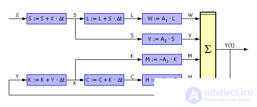
Assuming that the coefficients of the model are now known to us, we construct for the given example an implementation that simulates the behavior of the system described by the transfer function. To do this, we use the formula already obtained once:

or

The implementation of the model is shown in Fig. 5.4.

Fig. 5.4. Technical implementation of the transmission link after determination regression model coefficients

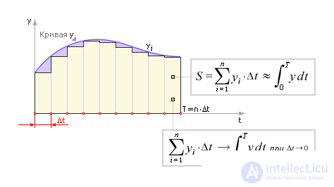
In the transition from integral to numerical summation, we used the method of rectangles. Having divided the area under the curve y into a row of rectangles of the same width Δ t (see Figure 5.5), we find that the area of ​​the i- th rectangle is equal to y _i · Δ t , and S is the sum of the areas of all n rectangles — approximately equal to the area under the curve (integral of the function y ). Obviously, the more accurate the approximation, the smaller the value of Δ t .

Fig. 5.5. Application of the rectangle method for numerical calculation of integrals