Lecture
Designing technological processes, checking project properties on a model, forecasting the progress of production, setting up a model for production processes, managing production has a number of features. The purpose of this lecture is to discuss the features arising from the modeling of production processes.
Suppose some production process is non-linear. This means that there is a non-linear relationship between the input X (with what is controlled) and the output Y (with what we observe). How to model such nonlinearity?
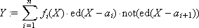
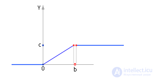
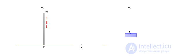
Example 1. Logic functions. First, consider the simple nonlinearity of the relay type and assume that the function Y ( X ) is reversible (see Fig. 31.1). Such dependencies are called static (the value at the input X is unique, regardless of the background of the process determines the value at the output Y ). Many manufacturing processes can be described in this way.
For example, suppose a dependency consists of three sections (see Figure 31.1). Often the characteristic feature of such dependencies is the presence in them of a section blocking the exit, a linear section and a section of saturation. The first section indicates that without supplying raw materials ( X = 0) to the input of the production process, one cannot hope for any result ( Y = 0). The second section indicates the fact that, by increasing the amount of raw materials at the entrance, we provide an increase in finished products at the output. And finally, it is clear that if there are a lot of raw materials ( Y >> 0), then any restrictions on the production process (for example, equipment performance, personnel qualifications, financial and energy resources) will still not allow processing all these raw materials and releasing appropriate quantity of products. In complex systems, such a site of saturation is necessarily present.
| |
| Fig. 31.1. The dependence of the relay type |
Please note that each of the sections can be easily described separately. Presented in Fig. 31.1 dependence is mathematically described by three functions. Three lines in the record mean that at each individual moment (that is, at a certain value of X ) one of the lines (first, second or third) is used from the description. That is, it is implied (but clearly not recorded) that the strings are connected by the sign OR . When dealing with computer technology and programming languages, where it is dangerous to remain silent, this construction is written to the string:
Y : = (0 for X ≤ 0) OR ( X · c / b for 0 < X ≤ b ) OR ( c for X > b ).
If the processes are analog, that is, if we are dealing with any (rational) values of X , the role of the operation OR is played by the “+” sign:
Y : = (0 for X ≤ 0) + ( X · c / b for 0 < X ≤ b ) + ( c for X > b ).
In fact: if conditions are mutually exclusive, then at any given time only one of the three conditions can be realized. It will give the required answer in the amount. From the remaining terms in the amount will come to zero. Adding the desired value with zeros will form the correct answer as a whole.
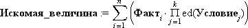
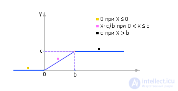
We now consider separately one of the constructions, for example, c for X > b . Its use means the following phrase (which is not written or uttered completely solely in order to save space and time): “if X is greater than b , then Y is assigned to c ”. We use the Heaviside unit function (see Fig. 31.2) to translate this phrase into a formal language. Recall that the value of a single function is 0 if its argument is less than or equal to 0, and equal to 1 if its argument is greater than 0.
| |
| Fig. 31.2. Heaviside Unit Function Y = ed (X) |
As a result, we obtain: Y : = c · ed ( X - b ). Check the resulting formula. Really:
Note that in our formula Y : = c · ed ( X - b ) the multiplication sign plays the role of a logical AND , because to get the final result we, first, need the value “ c ” AND , second, to be true ( ie, one) was the value of the expression ed ( X - b ).
As you can see, the verbal logical construction
if the condition , then the desired value : = fact
corresponds to a typical mathematical construction
Required_value : = Fact · ed ( Condition ).
IMPORTANT! So, the inequality turns into a single function (in mathematics, the single function is equivalent to the concept PREDICT), the logical OR is replaced with the addition sign, the logical AND is replaced with the multiplication sign. The “: =” sign expresses a causal relationship, linking the cause and effect explicitly. In the case of an implicit assignment of a function, the role of this sign will be played by the equal sign “=”.
Now we translate the second part of the expression, Y : = X · c / b with 0 < X ≤ b , into a formal language: Y : = X · c / b · ed ( X ) · ed ( b - X ). Note that the correct result will be obtained if three conditions are simultaneously met at the same time: ( X · c / b ) AND ( X > 0) AND ( X ≤ b ). We will do the same with the rest: Y : = 0 with 0 ≤ X. The formal translation is: Y : = 0 · ed (0 - X ).
Putting all three parts together, we have:
Y : = 0 · ed (0 - X ) + X · c / b · ed ( X ) · ed ( b - X ) + c · ed ( X - b ).
Please note that the first addend is generally not to write, since it is always equal to 0. It remains:
Y : = X · c / b · ed ( X ) · ed ( b - X ) + c · ed ( X - b ).
One more note. If we test the function at the point X = b , then it turns out that both the first term and the second one are simultaneously equal to 0, and the whole function will look like that shown in Fig. 31.3. This situation is called a snap. (Is there a snap between 0 · ed (0 - X ) and X · c / b · ed ( X ) · ed ( b - X )? If yes, for which X ? Check yourself.)
| |
| Fig. 31.3. Type of logical function with an error type slips in the description |
To avoid slips, it is necessary to write formulas more accurately:
Y : = X · c / b · ed ( X ) · not (ed ( X - b )) + c · ed ( X - b ).
Indeed, in this case, either not (ed ( X - b )) (from the first term), or ed ( X - b ) (from the second term) will necessarily be equal to 1, and the slip will disappear. Note that you can not enter the additional operation not ( q ), but use its analog: 1 - ed ( q ).
So, to summarize: if there are n segments in the dependency record, and X on the i- th segment satisfies the condition: a i < X ≤ a i + 1 , then we have:
Note. The function is unambiguous, that is, the same X always corresponds to the same Y. The convenience of such descriptions is that Y is calculated at any time for any X , it is enough to substitute the desired any value of X into the formula.
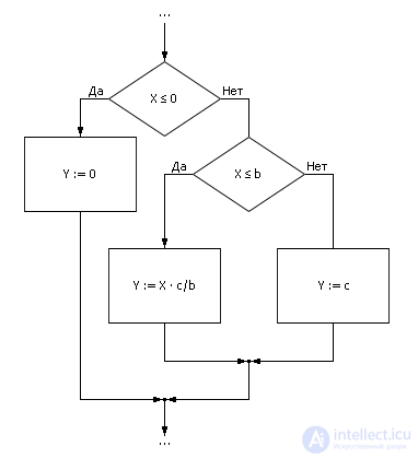
The type of recording depends on the system, which will have to perform such a recording. If the system does not understand the record, then it will not be able to execute it, and such a record is useless. A language is so dead and does not mean anything, since it does not serve as a means of communication, the transfer of information from one agent to another. (Looking ahead, we note that the language has other functions, for example, the ability to manipulate the objects that it describes, the calculus function.) For example, if the executor is an algorithmic machine, then the construction
Y : = X · c / b · ed ( X ) · not (ed ( X - b )) + c · ed ( X - b ).
will have the form shown in fig. 31.4.
| |
| Fig. 31.4. Algorithmic implementation of production models in the form of logical functions using conditional designs |
As you can see, there is a correspondence in the languages of description. Conditional construction in algorithms corresponds to a “multi-storey” formula in mathematics or construction
in a formalized modeling language. Or, using logical functions AND , OR , NOT :

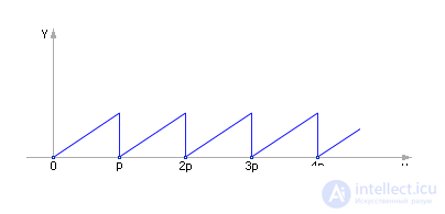
Example 2. The sawtooth generator (GPS). We construct a periodic sawtooth function (see Fig. 31.5) in two different ways.
| |
| Fig. 31.5. Type of dependence Y (X) for GPS |
Option 2.1. GPS based on the mathematical function mod . The well-known mathematical function mod ( X , a ) returns the remainder of division of X by a , and the remainder, as is well known, grows linearly with increasing X , and then becomes equal to 0 (when X and a become multiples), repeating this pattern periodically. In the Stratum 2000 environment, this is written as follows: Y : = X % a . The period and amplitude of the "saw" are governed by the values of X and a .
Option 2.2. GPS based on equation with memory . Y : = ( Y + d ) · ed ( p - Y ), where d is the step of change, p is the period. Suppose that at first Y is sufficiently small, therefore p > Y. If p - Y > 0, then for a positive argument the unit function returns 1, and the expression has the form: Y : = ( Y + d ) · 1, that is, Y increases at each step by the value d , which means it grows linearly.
Sooner or later, Y becomes equal to or greater than p , and the condition becomes p - Y ≤ 0. For a negative and zero argument, the unit function returns 0, which means the expression at this moment takes the form: Y : = ( Y + d ) · 0, then there is Y at this step is reset to zero, and the situation repeats: again, Y becomes small and begins to grow until it reaches the value of p . When applying the calculated value Y to the vertical coordinate of the oscilloscope, and to the horizontal coordinate of the value X , formed as X : = X + 1, one can see a saw with a period p (see Fig. 31.6).
| |
| Fig. 31.6. Scheme of the project in the environment Stratum-2000, implements a sawtooth generator based on the equation with memory |
Note. First, as you can see, in the expression Y : = ( Y + d ) · ed ( p - Y ), in order to calculate the next value of Y , you need to know the previous one. Therefore, it is said that this is a feedback equation or an equation with memory : to calculate the Nth value, it is required to calculate all previous values of the function in a number of steps. Secondly, the function was ambiguous. That is, with different initial data, the function graph will be different. The same X can correspond to different Y. This corresponds to a family of graphs generated by a differential equation. This entry is NEVER , since it does not contain the X value directly. Therefore, it is impossible to substitute an arbitrary value of X and immediately find out what Y will be equal to at this value. To determine the value of Y , it is necessary to go through (iterate) all Y values from 0 to the desired one.
The first variant of the record, Y : = X % a , represents to us an explicit dependence of Y on X. At any time, you can substitute any value of X and get the corresponding value of Y.
Each entry has its own advantages and disadvantages. It is not always possible to obtain an explicit record, since it is usually much easier to write down the law of the functioning of a system than to find its solution. But the obvious option also has the disadvantage that this is only one of the solutions, while the law itself contains potentially all of the many other possible solutions that are multivalued.
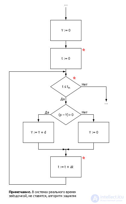
If you implement the expression Y : = ( Y + d ) · ed ( p - Y ) in the language of algorithms, then you need a cyclic construction (see. Fig. 31.7).
| |
| Fig. 31.7. Algorithmic implementation of the sawtooth model signal using cyclic construction |
There is a deep connection between a system with memory and a cyclic design, namely: a system with memory is a dynamic system , which corresponds in mathematics to a differential equation , step-by-step calculation of which on a computer requires a cyclic algorithm . If the solution of a differential equation can be found analytically, that is, to express the desired value depending on the others explicitly, then a cyclic construction is not needed, a linear structure algorithm is sufficient. But it will not actually be an equation, but an assignment, that is, a solution to the equation, more precisely, one of the solutions of the equation.
Example 3. The generator of rectangular pulses (GUI). In many applications, it is required to imitate the periodic opening and closing of some devices, gates, and channels for some time. For this it is convenient to use a pulse generator, which at the output would produce the values "0" and "1", that is, the generator of rectangular pulses. It is convenient to take for the generator parameters the frequency of changes from 0 to 1 and back and duty ratio - the ratio of the holding time at the output “1” to the time of the whole cycle.
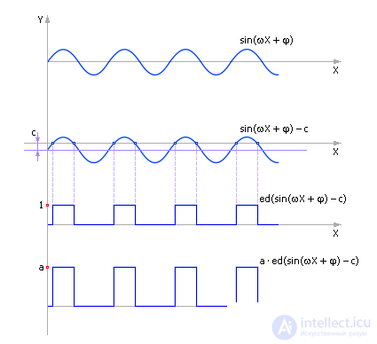
Option 3.1. GUIs based on periodic sine function . You can use several methods of modeling a square-wave generator with its own advantages and disadvantages. Let us first consider a generator using the properties of a periodic function, for example, a mathematical sine function (see. Fig. 31.8).
| |
| Fig. 31.8. Generating a sequence of rectangular pulses by means of a periodic function |
Y : = a · ed (sin ( ω · X + φ ) - c ), where ω is the frequency of the generator, specifying its period; φ - generator phase; a is the pulse amplitude; c - set parameter, duty cycle. The duty cycle indicates which part of the sine period Y will be equal to a , and which part of the period Y will be equal to 0. As long as sin ( ω · X + φ )> c , the unit function returns 1, Y = a ; as soon as sin ( ω · X + φ ) ≤ c , the unit function will return 0, Y = 0.
Again, note that this is an EXPRESS entry that determines the strengths and weaknesses of this option.
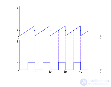
Option 3.2. GUI based on the equation with memory . Another option is to use a previously created sawtooth generator, which used a sequential calculation of values from point to point (equation with memory), to generate rectangular pulses.
Y : = ( Y + d ) · ed ( p - Y ), Z : = a · ed ( Y - c ), where d is the step of change; p is the period; a is the pulse amplitude; c - set parameter, duty cycle.
Since Y generates a sawtooth signal, it is sufficient to compare its value with the specified value c . If Y is c ≤ 0, then Z = 0, if Y is c > 0, then Z = a · 1. As a result, a periodic single signal is obtained. When feeding the oscilloscope to the vertical coordinate of the calculated Z value, and to the horizontal coordinate — the values of X formed as X : = X + 1, one can see a “fence” with a period p (see. Fig. 31.9).
This record has an implicit appearance that determines the advantages and disadvantages of this option.
| |
| Fig. 31.9. Generating a sequence of rectangular pulses using a memory expression |
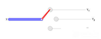
Example 4. Switch. A technological device often used in production processes is a switch whose purpose is to distribute some main flow (material, energy, information) to a number of private flows by switching the supply from one direction to another (see. Fig. 31.10). This allows you to divide the flow, change their direction.
| |
| Fig. 31.10. Switch layout |
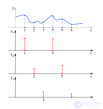
Suppose there is one input labeled X , and, for example, three outputs: Y 1 , Y 2 , Y 3 . Signal X is required to be broadcast on Y 1 at the first time instant, at Y 2 at the second time moment, and at Y 3 at the third time point, after which the process is repeated cyclically, starting again from Y 1 . (Of course, other variants of switches are possible.) The timing diagram of the distribution of the main flow to sub-streams by a discrete switch is shown in Fig. 31.11.
| |
| Fig. 31.11. Timing diagram of discrete work switch with one input and three outputs |
For this we need the Dirac delta function: Y = δ ( X ). This function returns 1 if its argument is 0, in other cases it returns zero (see. Fig. 31.12).
| |
| Fig. 31.12. Dirac Delta function Y = δ (X) (on the left - theoretical the view on the right is its approximate discrete analog) |
Using the delta functions, the expressions imitating the switch will look like this (in the entry below, the variable i plays the role of time t ):
i : = ( i + 1) · ed (2 - i )
Y 1 : = X · δ ( i - 0)
Y 2 : = X · δ ( i - 1)
Y 3 : = X · δ ( i - 2).
Thus, i , thanks to the first expression, runs cyclically the values 0, 1, 2, 0, 1, 2, 0, 1, 2, ... If i turned out to be 0, then δ ( i - 0) = 1 and Y 1 : = X · 1; moreover, δ ( i - 1) = 0 and Y 2 : = X · 0 and δ ( i - 2) = 0 and Y 3 : = X · 0.
If i turned out to be 1, then δ ( i - 1) = 1 and Y 2 : = X · 1, and δ ( i - 0) = 0 and Y 1 : = X · 0 and δ ( i - 2) = 0 and Y 3 : = X · 0.
If i turned out to be 2, then δ ( i - 2) = 1 and Y 3 : = X · 1, and δ ( i - 0) = 0 and Y 1 : = X · 0 and δ ( i - 1) = 0 and Y 2 : = X · 0.
To organize a cyclic switch, we needed a “saw” that we built earlier.
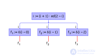
Note that it would be even better to do this: write expressions for the control system, where information signals i , f 1 , f 2 , f 3 are described:
i : = ( i + 1) · ed (2 - i );
f 1 : = δ ( i - 0);
f 2 : = δ ( i - 1);
f 3 : = δ ( i - 2).
Flags f i take values 0 and 1, as it should be in logical variables. The model of the information part of the project is shown in Fig. 31.13.
| |
| Fig. 31.13. Information management scheme signals for the switch |
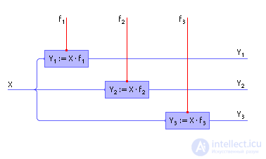
Then write separately the expressions for the material flows Y and X , which are overlapped by the control signals f i (see. Fig. 31.14):
Y 1 : = X · f 1 ;
Y 2 : = X · f 2 ;
Y 3 : = X · f 3 .
| |
| Fig. 31.14. Схема проекта, выполненного в среде Stratum-2000, реализующая коммутатор. Отражена часть проекта без формирователя флагов |
Переменные Y , X принимают действительные значения, как это и положено переменным, которые имитируют материальные потоки. Можно представить себе аналогию: поток X переходит в поток Y , если кран f открыт ( f = 1), или, наоборот, значения потока X не переходят на переменную Y , так как кран закрыт ( f = 0). Такая схема в дальнейшем более предпочтительна, так как отделяет материальную систему от информационной, делая проект более понятным и прозрачным (см. также пример 5 ниже).
Объединим информационную схему со схемой, имитирующей материальные потоки (см.рис. 31.15).
| |
| Fig. 31.15. Схема проекта «Модель коммутатора», представленного композицией информационной и материальной подсистем. Проект выполнен в среде Stratum-2000 |
In fig. 31.16 показано взаимодействие двух подсистем (информационной и материальной) между собой в общем виде, которого рекомендуется достигать в идеале для прозрачности процесса проектирования. Все зависимости и законы, касающиеся описания свойств материи и энергии, рекомендуется включать в состав модели материальных потоков (иногда в этой подсистеме дополнительно разделяют энергетические и материальные потоки), а законы измерения, управления, регулирования, формирования целей — включать в состав модели информационных сигналов.
| |
| Fig.31.16. Separation of the material and control models into separate subsystems |
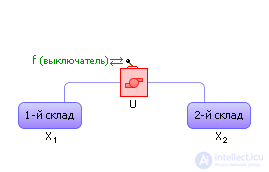
Example 5. Transportation of products from one node to another. A frequent case in production is the organization of transportation of products from one production unit to another. The node here will be understood as the aggregate of the warehouse and the transport body (for example, a vehicle, a canal). The warehouse stores products, the number of which may decrease or increase if the transport authority assumes their movement from node to node.
Suppose that on the first node there are X 1 products, and on the second - X 2 products. Denote as U the number of transported items per cycle. Then:
X 1 := X 1 – U · f ;
X 2 := X 2 + U · f .
In fig. 31.17 показана связь двух узлов транспортным каналом, осуществляющим перекачку изделий со склада одного узла на склад другого узла с производительностью U штук в единицу времени.
| |
| Fig. 31.17. Условное изображение модуля транспортировки с одного склада на другой |
Если флаг f равен 1, то U изделий уходит с первого узла и столько же в этот момент приходит на второй узел. Если флаг f равен 0, то переброски изделий не происходит, то есть они не вычитаются в первом выражении и не складываются во втором, а X 1 и X 2 остаются неизменными величинами.
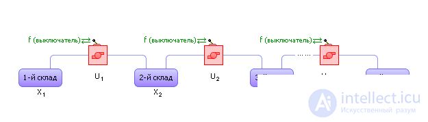
Если изделия необходимо транспортировать через цепь узлов (см. рис. 31.18), то, обозначая объемы перевозок между узлами U 1 , U 2 , …, U n – 1 , имеем:
X 1 := X 1 – U 1 · f ;
X 2 := X 2 + U 1 · f – U 2 · f ;
X 3 := X 3 + U 2 · f – U 3 · f ;
...;
X n := X n + U n – 1 · f .
| |
| Fig. 31.18. Схема транспортировки изделий через цепь складов |
Если задвижками f необходимо управлять по отдельности, то логично ввести переменные f i , управляя задвижкой в каждом узле отдельно.
Следует заметить, что данную модель для улучшения ее адекватности можно модернизировать:
X 1 := X 1 – U 1 · f · ed( X 1 );
X 2 := X 2 + U 1 · f · ed( X 1 ) – U 2 · f · ed( X 2 );
X 3 := X 3 + U 2 · f · ed( X 2 ) – U 3 · f · ed( X 3 );
...;
X n := X n + U n – 1 · f · ed( X n – 1 ).
Выражение ed( X i ) играет роль своеобразного флага разрешения транспортировки, запрещая ее в случае, если в узле нет изделий. Если такого флага нет, то возможны странные варианты переброски фиктивных изделий с узла на узел, например, появление отрицательных изделий.
One more note. На цифровой технике уравнения решаются с некоторым тактом. Если в течение такта окажется, что U i больше X i , то за такт из узла исчезнет больше изделий, чем в нем было, и количество изделий станет меньше нуля.
Во-первых, на это можно не обращать внимания, поскольку это погрешность численного расчета. Второй вариант — предотвратить все-таки такие коллизии. Для этого есть два способа. Первый состоит в том, чтобы уменьшить время d t такта расчета (до этого мы принимали его равным 1): X 1 := X 1 – U 1 · f · ed( X 1 ) · d t . Второй способ: вычитать и прибавлять значение U i , если U i < X i , или вычитать и прибавлять X i , если U i ≥ X i , то есть вычитать и прибавлять минимальное из двух чисел U i и X i : X 1 := X 1 – U 1 · f · ed( X 1 ) · ed( X 1 – U 1 ) – X 1 · f · ed( X 1 ) · not(ed( X 1 – U 1 )). В данной записи выражениеed( X i ), играющее роль своеобразного флага разрешения транспортировки, становится излишним, поэтому его можно опустить: X 1 := X 1 – U 1 · f · ed( X 1 – U 1 ) – X 1 · f · not(ed( X 1 – U 1 )). С учетом всего вышесказанного, напишем выражение для X 2 :
X 2 := X 2 + U 1 · f · ed( X 1 – U 1 ) + X 1 · f · not(ed( X 1 – U 1 )) – U 2 · f · ed( X 2 – U 2 ) – X 2 · f · not(ed( X 2 – U 2 )).
Если представить себе, что мы имеем дело с производственной технологической линией, то в качестве складов в этой цепочке выступают запасы незавершенной продукции (промежуточные склады в производстве), а роль транспортных артерий — станки, которые обрабатывают изделия, тем самым как бы «проталкивая» их с одного участка на другой.
Тогда U играет в этих выражениях роль производительности станков: чем больше U , тем больше изделий за одну единицу времени переходит с одного склада на другой, а X играет роль количества изделий на промежуточных складах в производстве. Таким образом, U характеризует динамику производственного процесса, а множество X — его статику. То есть X характеризует, сколько изделий находится в производстве в разной стадии готовности, а U — сколько изделий и с какой скоростью обрабатывается в каждый момент времени, как быстро перетекают изделия с узла на узел. Задавая различные значения U , можно имитировать различные производственные ситуации.
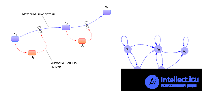
Иногда при описании производства задают закон движения U . Например, U = k · X . Логика действия такого закона состоит в том, что чем больше изделий X скапливается на складе, тем больше должна быть интенсивность их обработки U , чтобы избежать чрезмерного накопления изделий на промежуточных складах. Как ранее было описано, закон движения, в отличие от уравнений материального баланса, представляет собой информационный поток, это хорошо видно на рис. 31.19 .
| |
| Fig. 31.19. Два варианта изображения схемы модели технологической линии с информационными и материальными связями с различным уровнем детализации. Слева — обозначения по Форрестеру с разделением материальных и информационных потоков, справа — граф зависимостей переменных |
Можно задать и другие законы, например, U i := U i + k · ( X i – X i + 1 ). Логика этого закона состоит в том, что если на i + 1-ом складе затоваривание ( X i + 1 > X i ), то надо притормаживать U i , если недостаток, то есть X i + 1 < X i , то разгонять производительность данного узла.
Измерительная часть системы управления может фиксировать общее количество изделий P 1 на всех складах, их суммарную стоимость P 2 , общую производительность станков P 3 , неравномерность распределения изделий в производстве P 4 , выполнение плана X z — P 5 и так далее:
P 1 = X 1 + X 2 + X 3 + … + X n ;
P 2 = X 1 · c 1 + X 2 · c 2 + X 3 · c 3 + … + X n · c n ;
P 3 = U 1 + U 2 + U 3 + … + U n ;
P 4 = abs( X 1 – X 2 ) + abs( X 2 – X 3 ) + … + abs( X n – 1 – X n );
P 5 = X n – X z .
По данным показателям можно настраивать регуляторы в производстве, добиваясь приемлемых значений у этих показателей.
С помощью такого подхода, используя логические комбинации ( И , ИЛИ , НЕ ) и условия, отражаемые единичными функциями, можно описать разделения, слияния потоков, переход партий, сборку, брак, помехи, задержки, переход изделий с линии на линию, и вообще любую производственную топологию.
Задачи, которые можно решить на такой модели:
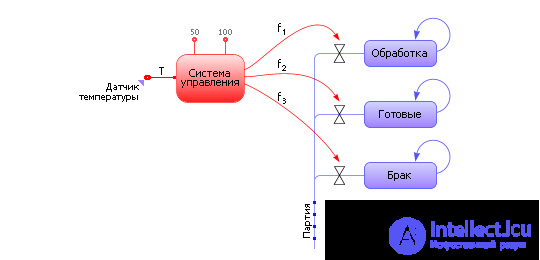
Пример 6. Обработка партии изделий в термической печи. Рассмотрим обработку партии изделий в термической печи. Если температура в печи до 50 градусов, то партия снова поступает в обработку. Если температура в печи между 50 и 100 градусами, то партия уходит на склад готовых изделий. Если температура в печи больше 100 градусов, то партия поступает в брак.
The block of information signals has the form:
f 1 : = ed (50 - T );
f 2 : = not (ed (50 - T )) · ed (100 - T );
f 3 : = not (ed (100 - T )).
Block imitation of material processes:
Arr: = Party · f 1 ;
Ready: = Ready + Batch · f 2 ;
Marriage: = Marriage + Party · f 3 .
Pay attention: on the model diagram (Fig. 31.20), all possible and essential for the process conditions “ed (Condition)” are separately formed, information signals ( f 1 , f 2 , f 3 ) are separately formed, material flows are described separately.
| |
| Fig. 31.20. Diagram of the model “Processing of products in a heat-treatment furnace” |
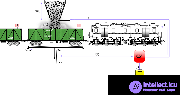
Example 7. Train loading. Consider the process of loading a train consisting of an electric locomotive and three cars attached to it (see fig. 31.21). Above the first car is a bunker from which the load is poured. The car stands on the scales, measuring the mass of the loaded cargo. The capacity of the cars is set and known to the control system from the directory in the database of ACS. The control system (SU) must determine the moment (and issue a control signal to the electric locomotive) when to put the next car for loading. After loading the last car, close the hopper flap.
| |
| Fig. 31.21. Train loading and control system |
Let U ( t ) be the current load of the car, the value on the scales; V ( t ) is the intensity of the cargo entering the car from the bunker, the quantity per cycle; i - car number (1, 2, 3); E ( i ) is the load capacity of the i- th car (set); X ( t ) is the level of raw materials in the bunker; f - signal to the locomotive driver: “pull the train through one car”.
Expressions that simulate loading and control system responses should simulate the loading process (laws of changes in U ( t ), X ( t ) and V ( t )), ACS signals ( f and i ).
U ( t ): = ( U ( t ) + V ( t )) · ed ( E ( i ) - U ( t )) - the loading of the car increases if the car is not full, and stops and is reset to zero if the car is loaded up to norm E ( i );
f : = not (ed ( E ( i ) - U ( t ))) - a signal to the locomotive driver: “drive the train”;
i : = i + f - the car counter increases at the moment of pulling in the train;
X ( t ): = X ( t ) - V ( t ) - the level of raw materials in the bunker decreases;
a : = k · X ( t ) - the lower the level of X , the slower the raw material is poured out, since the upper layers put less pressure on the lower ones;
V ( t ): = a · B is the intensity of the cargo entering the car from the bunker;
B : = ed (3 - i + 1) · ed ( X ( t )) - the raw material enters the car, if its number is not greater than the third one. And there is raw material in the bunker.
On the basis of the constructed model, it is possible to solve a number of problems, for example, determine the time for which the entire train will be loaded, or find out other other issues. In general, what task will be solved on a model depends largely on the goals of the person using this model.
Example 8. Trigger. Often, control of information signals requires a trigger. The truth table of the trigger is presented in table. 31.1.
| Table 31.1. Trigger Truth Table | |||||||||||||||||||||||||||||||||||||||||||
| |||||||||||||||||||||||||||||||||||||||||||
This device, as can be seen from the table. 31.1, is easily described by logical functions, but at the same time it is a system with memory (inside the trigger there is a feedback circuit, mathematically: Q : = F ( R , S , Q ), see Fig. 31.22).
| |
| Fig. 31.22. Symbol trigger on charts |
Imagine a trigger model using the logical functions of its state. In tab. 31.1 select all rows with Q = 1 (column “New state of trigger, exit”). There are three of them. We write three situations through the operation OR : Q : = c 1 OR c 2 OR c 3 . Each situation, in order for a line to produce 1 at the output, must be a SIMULTANEOUS combination of R , Q , S signals, that is, R AND Q AND S. If the input signal in the line is 1, then the variable must be taken "as is", if it is 0, then invert with the function NOT. For example, the string
|
gives: NOT ( R ) AND NOT ( Q ) AND S And Q , or, using the functions in the record, as they are usually implemented in formal languages, we have: not ( R ) · not ( Q ) · S · Q , or another variant : and (and (not ( R ), not ( Q )), and ( S , Q )). The whole table in the form of a logical function is described as:
Q : = (not ( R ) · not ( Q ) · S ) OR (not ( R ) · Q · not ( S )) OR (not ( R ) · Q · S ).
In tab. 31.2 for reference, the values of commonly used logical functions AND , OR , NOT are given . Finally, citing similar ones, putting them out of the brackets and using a formal, generally accepted language record, we get:
Q : = and (not ( R ), or ( S , and ( Q , not ( S )))).
| Table 31.2. Logical values functions AND, OR, NOT | |||||||||||||||||||||||||
|
Example 9. START STOP or Trap. Now suppose that we need to simulate such a process, which begins when a certain signal Y is executed, then some time T p passes and stops by itself after the passage of such time. If during the process the signal Y is received again, then the process ignores such signal Y. If the Y signal comes again when the process is stopped, then the process is ready to accept the signal and respond to it again.
This design is called a trap because the model temporarily captures the input signal and does not respond to other input signals during this time. With the help of such structures, they often imitate the process of processing products in separate nodes of the processing line. The product falls into a knot, as if it were a trap, and leaves it only after a certain time. During this time, the node is busy and not ready to receive other products (input signals). It turns out that the product is occupied by the node, and the node is occupied by the product.
Let's call the flags for clarity:
“Can_start” - the flag is set to 1 if the process can be started, and the process can be started if the Y signal has arrived And the process is not going now;
“Process_id” - the flag is set to 1 if the process occurs, that is, it has already begun And it has not ended yet. The process goes on, if you can start the process OR if the process is already underway And it has not stopped yet;
“Stop” - the flag is set to 1 if it is necessary to stop the process, and this happens if the process is already or not yet OR the time of the process is over.
Now we write the equations according to logic (the signs used are & (AND) and | (OR)):
You can start: = ed ( Y ) & not (Process_who);
Process_it: = Can_start | (Process_id & not (Stop));
t : = ( t + h ) · ed ( T p - t ) · Process_tit;
Stop: = not (Process_sit) | not (ed ( t )).


Comments
To leave a comment
System modeling
Terms: System modeling