Runge Kutta Method

The Runge-Kutta method is used to calculate standard models quite often, since with a small amount of calculations it has the accuracy of the method Ο 4 ( h ).

To build a difference integration scheme, we use the decomposition of the function

in taylor row:

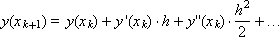
Replace the second derivative in this decomposition with the expression

Where

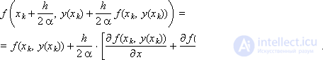
Moreover, Δ x is selected from the condition for achieving the highest accuracy of the written expression. For further calculations, we replace the value of “ y with a tilde” by decomposing into a Taylor series:

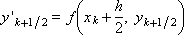
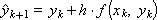
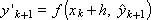
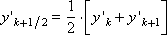
For the original equation (1) we construct a computational scheme:

which we transform to the form:

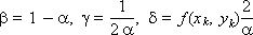
We introduce the following notation:

These symbols allow you to write the previous expression in the form:

It is obvious that all entered coefficients depend on the value of Δ x and can be determined through the coefficient α , which in this case plays the role of a parameter:

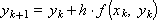
Finally, the Runge-Kutta scheme takes the form:

The same scheme in the form of a difference analogue of equation (1):

When α = 0, we obtain as a special case the already known Euler scheme:

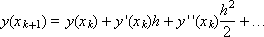
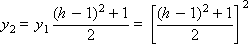
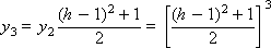
When α = 1:

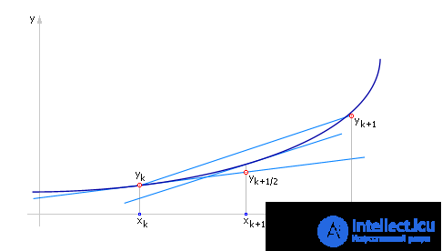
When α = 1, the calculations at the next integration step can be considered as a sequence of the following operations.

1. An expression that represents the half-step of integration according to the Euler scheme is calculated, that is, an approximate value of the unknown function is determined at the point x k + h / 2:

   

2. For the same intermediate point is the approximate value of the derivative:

   

3. The refined value of the function is determined at the end point of the entire step, and according to the Euler scheme with the derivative value calculated at the previous step:

   

Geometric constructions (see Fig. 15.1) show that the solution obtained in this sequence lies “closer” to the true one than that calculated by the Euler scheme, that is, one should expect a higher accuracy of the solution obtained by the Runge-Kutta method. Earlier, we called this scheme the “modified Euler method.”

Fig. 15.1. Illustration of calculation on a step by the Runge-Kutta method when the value of the parameter α = 1

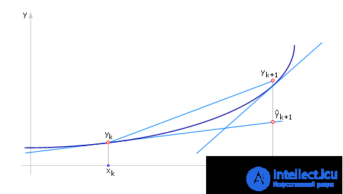
Now consider the scheme for α = 0.5 (the geometric interpretation of the result is shown in Fig. 15.2).

1. The full step of the Euler method is performed in order to determine the approximate value of the unknown function at the end of the integration segment:

   

2. For the same point, an approximate value of the derivative is calculated:

   

3. The average value of the two derivatives determined at the ends of the segment is found:

   

4. Calculates the value of the desired function at the end point of the entire step of the Euler scheme with the average value of the derivative:

   

Fig. 15.2. Illustration of calculation on a step by the Runge-Kutta method at value α = 0.5

Sometimes the resulting expression is called the Euler-Cauchy scheme (method). Geometrically, it is clear that the result obtained in this way must also be “closer” to the true solution than that obtained by the Euler scheme.

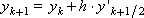
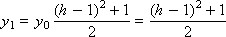
Example. Solve the equation d y / d x = - y , y (0) = 1 using the Runge-Kutta method.

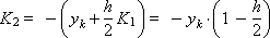
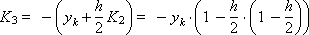
Since the right side of the differential equation has the form: f ( x , y ) = - y , the scheme of the method with α = 0.5 is represented as follows:

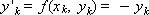
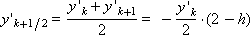
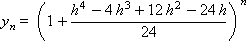
Construct a sequence of values ​​of the desired function:

...

The results of the obtained numerical solution for the value of the argument x = 10 with different integration steps are given in Table. 15.1. Three valid significant digits are obtained for step h = 0.01.

Let us estimate the error of approximation of equation (1) by the difference scheme of the Runge-Kutta method. We substitute the exact solution into the difference analog of the original differential equation and calculate the residual:

Substitute the decomposition of functions

in the resulting expression:

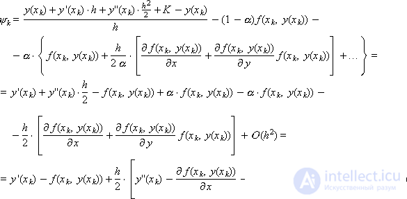
Given equation (1), as well as the expression for the derivative

finally, we obtain that ψ k = ( h 2 ), that is, the Runge-Kutta method, regardless of the value of the parameter α , has the second order of approximation.

Methods of Runge-Kutta of the third and fourth orders

Let us consider two different Runge-Kutta schemes designed for the numerical solution of ordinary differential equations of the first order and having the third order of approximation:

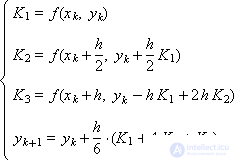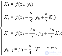And two Runge-Kutta schemes with the fourth approximation order:

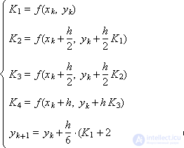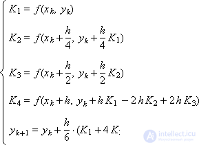Example. Solve the fourth order Runge – Kutta method by the equation d y / d x = - y , y (0) = 1.

In accordance with the above ratios, we determine the coefficients:

Construct a sequence of values ​​of the desired function:

...

The results of the obtained numerical solution for the value of the argument x = 10 for various integration steps are given in Table. 15.2. Three valid significant figures are obtained for step h = 0.25.

Comparison of tables 15.1 and 15.2 with solutions of the same problem allows us to conclude that a higher degree of approximation of a differential equation by a differential analog allows to obtain a more accurate solution for a larger step and, therefore, fewer steps, that is, leads to a decrease in the required computer resources .

To date, for a rough calculation, calculations are made by the Euler method, for exact calculations - by the Runge-Kutta method.