Dynamic systems

In previous lectures, we considered static models, that is, the case when one experiment does not depend on another. We can say that the system did not have a memory. That is, at whatever point in time we measure the value of the output value, with the same value of the input signal, the result was the same. If each time the value at the output, for the same input value, is different, that is, it depends on the sequence in which the input values ​​were supplied, then we are dealing with a dynamic system .

Dynamic systems, unlike static ones, remember their past state, that is, they have memory. Therefore, in the record of the model of dynamic systems there is a derivative connecting the past state of the system with the present. The more memory the system has, the more states from the past affect the present, the greater the degree of the highest derivative used in recording the model. This lecture deals with dynamical systems.

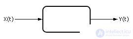
Task 1. At the input and output of the black box (Fig. 4.1) there are dependencies of the parameters X and Y on time t . The challenge is to adequately identify the black box.

Fig. 4.1. Black box containing dynamic the system. Symbol

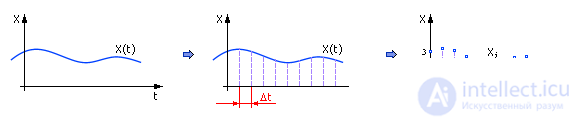
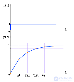
The graphs of dependencies X ( t ) and Y ( t ) can be very different, for example, such as shown in Fig. 4.2.

Fig. 4.2. Time dependencies - input and output signals

Since the simulation of systems involves numerical calculations on a computer, the analog signal is transferred to a discrete form. To do this, the source signal is sampled at a certain frequency, as shown in Fig. 4.3.

Fig. 4.3. Discretized time signal

From these data, a table of readings is constructed (see Table 4.1, where Δ t = 0.1).

A set of variable values ​​in a table, ordered in time, is often called a dynamic series. Naturally, some of the information in this operation is lost. The smaller the distance between samples, the greater the sampling rate, the less information is lost. The sampling rate is taken so as not to lose the high-frequency components in the signal, separate peaks (see also “Lecture 08. Model of a dynamic system in the form of a Fourier representation (object model)”).

Any dynamic system is characterized by a number of parameters. Usually (most often) parameters are called coefficients for derivatives (first, second, etc.) in the model record. The greater the degree of the higher derivative present in the model record, the greater the order of the dynamic system, the deeper its memory, and the more coefficients (parameters) it is necessary to determine in order to identify the system.

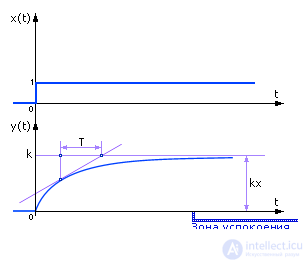
How to determine the parameters of a dynamic system? First, we must estimate the order of the dynamical system: it coincides with the degree of the greatest derivative of Y with respect to t . Suppose that a single signal X ( t ) was applied to the input of the system, which was previously in zero initial conditions, as shown in Fig. 4.4.

Fig. 4.4. Typical input and output signal for the first order system

Explain the meaning of the schedule. Under zero initial conditions, if there is no input signal, the output signal is zero, and the system is said to be at rest. If you send a single (test) signal to the input and keep it at the input long enough, then the system at the output will try to obey it, will start to deviate from the zero state. It is expected that the output system should reach the value of k x , that is, increase the signal x by a factor of k ( k is the gain of the input signal). But, as you can see, this does not happen immediately, but with some delay, the output signal increases gradually, inertia. How inertia the system reacts depends on the parameter T. The system will reach the k x value at the output and will hold this signal as long as a single signal is held at the input. The transition from zero to k x occurs in time. The transition is a dynamic process, that is, there is a change in the signal that is described by the derivative, and the output is less than the input by some value f :

y = k x - f (d y / d t ).

When the system reaches the output value equal to k x , then there will be no changes, the value of the derivative will be equal to zero. y = k x .

y = k x - a special case of the inertial link.

If an output exponential signal is observed, the system will be called a first-order system (or a first-order link). One derivative is enough to describe it (and one integral will be present in the solution of the model):

Such a system has two parameters - T and k .

Note that one integral of linear dynamical systems always "generates" one exponent, a double integral is the sum of two exponents, and so on.

To determine whether a curve is an exponential, a tangent is drawn at each of its points until it intersects with a steady-state line (in Fig. 4.4, this is the line y ( t ) = k ); if the curve is an exponent, the value of T at any point will be constant.

It is possible to determine T using the graph as follows. Draw a line parallel to the t axis at 0.95 k . From the point where this line crosses the exponent, lower the perpendicular to the t axis. The segment from 0 to the point of intersection of the perpendicular with the axis t will be equal to 3 T.

T characterizes the inertia of the system (memory). With a small value of T, the system weakly depends on the prehistory and the input instantly causes the output to change. With a large value of T, the system responds slowly to the input signal, and with a very large value of T, the system produces a constant output signal, practically not responding to input influences.

The coefficient k characterizes the ability of the system to increase (when k <1 - to attenuation) the level of the input signal. To determine the coefficient k on the graph, it suffices to wait for the signal at the system output to calm down and calculate the ratio of the output signal level to the input level. Mathematically, this means that all the terms containing derivatives are zero (the system calmed down, there is no movement), and the remaining term Y = k · X determines the value of k .

First order link

A first-order link has two parameters: inertia T and gain k = Y ( t = ∞) / X.

The more derivatives are taken into account in the model record, the more we deal with the link of a higher order, the more coefficients for derivatives should be determined.

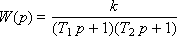
We introduce the concept of a transfer function as a model of a dynamic system. By definition, the transfer function is the ratio of the output to the input:

W = Y / X.

The transfer function of the link of the first order is:

W = k / ( T p + 1),

where " p " is a symbol of differentiation, identically equal to " d / dt ". The symbol “ p ” is also called an algebraized differentiation operator. Then, using the definition of the transfer function, we have:

Y / X = k / ( T p + 1).

Next we get:

( T p + 1) · Y = k · X

or

T · d Y / d t + Y = k · X

or

T · Δ Y / Δ t + Y = k · X.

In difference form, the equation can be written as

T · ( Y _{i + 1} - Y _i ) + Y _i · Δ t = k · X _i · Δ t .

Or, expressing the present through the past:

Y _{i + 1} = A · X _i + B · Y _i .

Here A = k · Δ t / T and B = 1 - Δ t / T are weighting factors. A indicates the weight of the X component, which determines the influence of the outside world on the system, B indicates the weight of the Y component, which determines the memory of the system, the influence on its history behavior.

In particular, if B = 0, then Y _{i + 1} = A · X _i , and we are dealing with the inertialess system Y = k · X , which instantly reacts to the input signal and increases it by a factor of k .

If the coefficient B = 0.5, that is, 1 - Δ t / T = 0.5 or Δ t / T = 0.5, then we get that the coefficient A = k · Δ t / T = k · 0.5 and, therefore, Y _{i + 1} = 0.5 · k · X _i + 0.5 · Y _i . With a constant (single) input signal X , a graph will be obtained, as in Fig. 4.5.

Fig. 4.5. Reaction of the first order per unit input for discrete case

The exponent shown on the graph, with large n (in the limit n = ∞), tends to the value of the input (single) signal X multiplied by the gain factor k , which is confirmed by the calculation:

Y _{n + 1} = 0.5 · k · X _n + 0.5 · Y _n = 0.5 · k · X _n + 0.5 · (0.5 · k · X _{n - 1} + 0.5 · Y _{n - 1} ) =
= ... = (0.5 ¹ + 0.5 ² + ... + 0.5 ^{n + 1} ) · k · X ₀ + 0.5 ^{n + 1} · Y ₀ = 1 · k · X ₀ .

Recall that the expression (0.5 ¹ + 0.5 ² +… + 0.5 ^{n + 1} ) is a geometric progression, the sum of which when n = ∞ is 1. And the expression at Y ₀ 0.5 ^{n + 1} turns into 0 when n = ∞.

If we further strengthen the influence of the past ( B = 1), the system will begin to integrate itself (the output is fed to the system input), adding the input signal all the time, which corresponds to an exponential unlimited growth of the output signal: Y _{i + 1} = A · X _i + Y _i . In the sense of this corresponds to a positive feedback. When B = –1, we have a model: Y _{i + 1} = A · X _i - Y _i , meaning corresponding to negative feedback. When defining a model, it is required to find unknown coefficients k and T.

Link of the second order (oscillatory link)

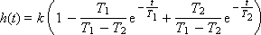
Such links are described by a differential equation of the form:

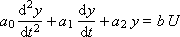
If a unit has a Heaviside function of time 1 [ t ] at the input, under zero initial conditions of the system, then the response at the output will be called a transition function (or transition characteristic), which is often referred to as h ( t ). Signal 1 [ t ] is, in a sense, a reference test signal. There are other reference test signals. For example, an infinite impulse of zero length (Dirac delta function), a harmonic signal, periodic rectangular pulses.

Laplace transform this equation:

a ₀ · p ² · Y ( p ) + a ₁ · p · Y ( p ) + a ₂ · Y ( p ) = b · U ( p )

or otherwise:

( a ₀ · p ² + a ₁ · p + a ₂ ) · Y ( p ) = b · U ( p ).

Define the transfer function of the link:

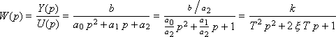
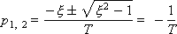
If we write an equation without an input (zero input effects U = 0) and reduce Y , that is: T ² p ² + 2 ξ T p + 1 = 0, then such an equation will be called characteristic, since it characterizes only the internal properties of the link. Notice that the link entry contains three parameters:

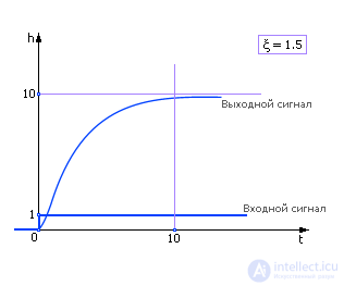
Depending on the value of ξ, second-order links are classified by type:

• ξ = 0 is a conservative link of the second order;
• 0 < ξ <1 is a second-order oscillatory component;
• ξ ≥ 1 is a second-order aperiodic link.

2nd order aperiodic link ( ξ ≥ 1)

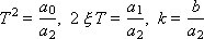
The characteristic equation of the link is as follows:

T ² p ² + 2 ξ T p + 1 = 0.

And it has real negative roots:

This link can be presented in the form of series-connected links with different time constants:

Then, at T ₁ > T _{2, the} transient response of the link is:

That is, the solution contains damped exponents. Typical behavior of a link with such parameters is shown in fig. 4.6.

Fig. 4.6. Aperiodic Reaction per unit input

In the particular case when ξ = 1, both roots will be the same, negative:

2nd order oscillatory link (0 < ξ <1)

The characteristic equation of the link is as follows:

T ² p ² + 2 ξ T p + 1 = 0.

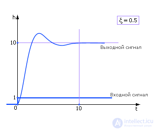
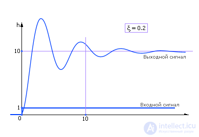
Roots are different, complex-conjugate, with a negative real part:

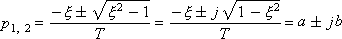
, where a = - ξ / T , b = sqrt (1 - ξ ² ) / T.

Since the roots are imaginary, the vibrational component is present in the link behavior. It is for this peculiarity of behavior that the link has been called oscillatory (see Fig. 4.7 and Fig. 4.8).

Fig. 4.7. Oscillatory response to input single signal (ξ = 0.5)

Fig. 4.8. Oscillatory response to input single signal (ξ = 0.2)

From the graphs it can be seen that with increasing ξ, the vibration of the link decreases, disappearing at ξ ≥ 1

The transition function of the link is:

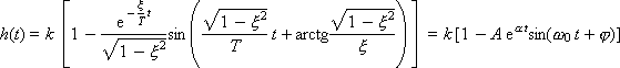
Where

For small ξ, the value of A approaches 1, and the value of φ - to 90 °. According to the physical meaning, ω ₀ is the natural frequency of oscillation.

2nd order conservative ( ξ = 0)

The characteristic equation of the link is as follows:

T ² p ² + 1 = 0.

The roots are the same, complex-conjugate, with zero real part:

Since the roots are purely imaginary, the link behavior is continuous oscillations ( ξ = 0), see fig. 4.9.

Fig. 4.9. Reaction of an oscillatory link to an input single signal (ξ = 0)

The transition function of the link has the form: h ( t ) = k · (1 - cos ( t / T )).

From the graph experimentally, you can determine a single parameter T = T ₀ / (2 · π ).