Lecture
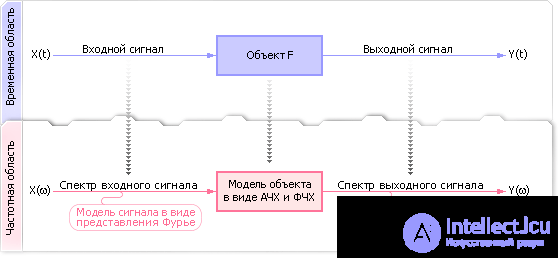
Suppose there is an input dynamic signal X ( t ) and an object F that converts this signal into output Y ( t ) (see Fig. 8.1). If the object is described by differential equations, then this transformation is the integration of the input signal and the calculation of Y ( t ). Integration, as previously shown, is an operation that requires significant computational resources and has a significant error in the implementation on digital machines.
| |
| Fig. 8.1. Dynamic object simulation scheme when moving from the time domain to the frequency domain |
If we go from the description of the input signal in the time domain to the description in the frequency domain (see Fig. 8.1), and from the differential equations go to the frequency response of the object, that is, in fact, replace the signal with the frequency model of the signal, and the object with the frequency model object, from a computational point of view, the signal conversion process is simplified. Of course, the result will also be the frequency model of the output signal, which will have to be converted into the time domain Y ( t ) to get the final answer. The process of such conversion from the frequency domain into the time domain and back is called the Fourier transform (there are other transformations). For those objects for which their model is known in the frequency domain, such an approach is quite simply implemented on a computer and allows you to achieve any pre-specified accuracy.
The object model in the frequency form is called the transfer function or frequency response (amplitude-frequency characteristic). Objects for which the frequency response is known are usually called typical links (amplifying element, aperiodic, oscillatory, etc.). Let, for example, the characteristic of an object in the frequency domain is as follows (see Fig. 8.2).
| |
| Fig. 8.2. AFC (possible view) |
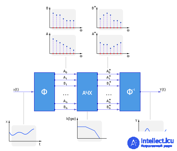
The amplitude-frequency characteristic (AFC) shows how far the object is outputting the corresponding harmonic. The value of k i characterizes the amplification factor of the harmonic signal at a certain frequency ω i .
Simulation of a signal passing through an object in this form consists in multiplying the harmonic coefficient A i with the frequency ω i of the input signal X ( t ) by the gain k i at the same harmonic with the frequency ω i in the frequency response: A i * = A i ( ω i ) · K i ( ω i ). (For coefficient B, the transformation is similar.) The result is the coefficient A i * of the output harmonics of a given frequency ω i . The procedure is performed for all frequencies represented in the input signal and frequency response. After obtaining the spectrum of the output signal, you can restore the signal as a time dependence using the inverse Fourier transform formula.
We note the main thing : the simulation of signal passing through a dynamic object was reduced to the operation of multiplying two variables, more precisely, the operation of elementwise multiplication of the vector of some variables by the vector of other variables.
The transformation scheme is shown in Fig. 8.3.
| |
| Fig. 8.3. Diagram of the signal conversion procedure using the Fourier method |
If the time signal passed through a link that is represented by a differential equation in the time domain, then it would have to be integrated, which, of course, leads to errors in the result. In the frequency domain, it is sufficient to multiply the values of the coefficients of the Fourier series of the signal and the link at the same frequencies. It is obvious that the advantage of the method is the replacement of the differential equations of the model for algebraic ones. Of course, this approach can be used only for objects that have a known form of the transfer function . (By the way, for unknown cases, the frequency response can be obtained by numerical decomposition in a row .)
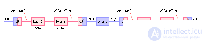
In the process of modeling a set of objects to convert a signal (for example, extended paths of electronic devices) sometimes it is necessary to apply the direct and inverse Fourier transform repeatedly. In practice, sequential blocks are often called cascades.
Suppose we have a radio-electronic device (REU), consisting of 5 blocks (see. Fig. 8.4). Blocks 1, 2, 4, 5 are linear and are represented by corresponding known frequency response; block 3 is non-linear, therefore the frequency response for it is unknown. An example of a linear block is an aperiodic link, an oscillatory link, and so on (see Lecture 05. Dynamic regression models defined as a transfer function). An example of a nonlinear block can serve as a signal limiting device (cutoff) in amplitude.
As can be seen from fig. 8.4, first, the input signal X ( t ) is transferred by the direct Fourier transform to the frequency domain and passes in the form of a spectrum through the frequency response 1 and 2 of the linear block, then the inverse Fourier transform transforms the signal after 2 blocks to the time domain. We pass a non - linear block 3 in the time representation. The result of operation of block 3 is again transformed by direct Fourier transform into the frequency domain and passing through the frequency response of blocks 4 and 5. At the end, the resulting spectrum is transformed using the inverse Fourier transform into the time domain, the signal type, Z ( t ), is the result of the simulation.
| |
| Fig. 8.4. An example of modeling a path containing non-linear blocks using the Fourier method |
The method we reviewed is one of the fastest. This is due to the replacement of the operations of integration and differentiation occurring in models of dynamic links by the operations of addition and multiplication during the transition to the frequency domain. Such a procedure ensures the accuracy and speed of the model.
For the method, it is important how often you sample the signal when decomposing into a Fourier series. If the sampling frequency is low, that is, the samples in the signal rarely follow, with large intervals, then a part of the signal remains lost, since between the samples there may be a sharply increased and fallen peak, information about which will disappear. That is, it is said that a low sampling rate cuts off high frequencies in the signal. (Peak - this is the high-frequency component, which may be lost).
According to Kotelnikov's theorem, in order not to lose the corresponding harmonic, it is required to sample a signal with a frequency of not less than 2 times greater than the highest frequency represented in the analog signal:
2 W max ≤ W p. ,
where W is disc. = 1 / Δ t disc. - sampling frequency, W max - the maximum frequency present in the signal.


Comments
To leave a comment
System modeling
Terms: System modeling