Lecture
In previous lectures, we learned to imitate the onset of random events. That is, we can play - which of the possible events will come and in what quantity. To determine this, it is necessary to know the statistical characteristics of the occurrence of events, for example, the probability of occurrence of an event, or the probability distribution of different events, if the types of these events are infinitely many.
But it is often still important to know when a particular event in time will occur.
When there are many events and they follow each other, they form a stream . Note that the events in this case should be homogeneous, that is, they resemble each other. For example, the emergence of drivers at the gas station wishing to fill your car. That is, homogeneous events form a series. It is assumed that the statistical characteristic of this phenomenon (intensity of the flow of events) is set. The intensity of the flow of events indicates how much on average such events occur per unit of time. But exactly when each specific event will occur must be determined by modeling methods. It is important that when we generate 1000 events for 200 hours, for example, their number will be approximately equal to the average intensity of occurrence of events 1000/200 = 5 events per hour, which is a statistical value characterizing this stream as a whole.
The intensity of the flow is in a sense the expectation of the number of events per unit of time. But it may actually happen that 4 events will appear in one hour, 6 events in another, although on average 5 events per hour will appear, therefore one quantity is not enough to characterize the flow. The second value characterizing how large the scatter of events is in relation to the expectation is the variance, as before. Actually it is this value that determines the randomness of the occurrence of an event, the weak predictability of the moment of its occurrence. We will tell about this value in the next lecture.
So.
The flow of events is a sequence of homogeneous events occurring one after the other at random intervals of time. On the time axis, these events appear as shown in Fig. 28.1.
|
|
| Fig. 28.1. Random event stream |
|
An example of a stream of events is the sequence of moments of contact with the runway by planes arriving at the airport.
The flux intensity λ is the average number of events per unit of time. The intensity of the flow can be calculated experimentally using the formula: λ = N / T n , where N is the number of events that occurred during the observation time T n .
If the interval between events τ j is equal to a constant or is defined by a formula in the form: t j = f ( t j - 1 ), then the flow is called deterministic. Otherwise the flow is called random.
Random streams are:
It is customary to take the Poisson flow for the standard flow in modeling .
Poisson flow is an ordinary flow without aftereffect.
As previously stated, the probability that m events occur over the time interval ( t 0 , t 0 + τ ) is determined from Poisson’s law:

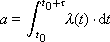
where a is the Poisson parameter.
If λ ( t ) = const ( t ), then this is a stationary Poisson flow (the simplest). In this case, a = λ · t . If λ = var ( t ), then this is a non-stationary Poisson flow.
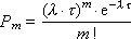
For the simplest flow, the probability of occurrence of m events in time τ is equal to:
The probability of non-occurrence (that is, none, m = 0) of an event in time τ is equal to:
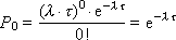
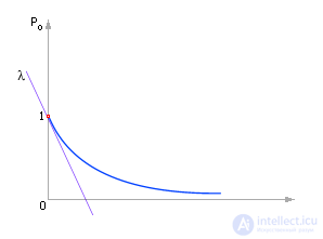
Fig. 28.2 illustrates the dependence of P 0 on time. Obviously, the longer the observation time, the less likely that no event will appear. In addition, the greater the value of λ , the steeper the graph, that is, the probability decreases faster. This corresponds to the fact that if the intensity of the occurrence of events is high, then the probability of non-occurrence of the event quickly decreases with the observation time.
|
|
| Fig. 28.2. The graph of the probability of failure no event in time |
The probability of occurrence of at least one event ( P HB1C ) is calculated as follows:

since P HB1C + P 0 = 1 (either at least one event appears, or no one appears, - no other is given).
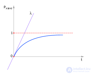
From the graph in fig. 28.3 it is clear that the probability of the occurrence of at least one event tends to be unity with time, that is, with appropriate long-term observation of the event, such an event will happen sooner or later. The longer we observe an event (the more t ), the greater the likelihood that an event will occur - the graph of the function monotonously increases.
The greater the intensity of the occurrence of an event (the larger λ ), the faster this event occurs, and the faster the function tends to unity. In the graph, the parameter λ is represented by the slope of the line (the slope of the tangent).
|
|
| Fig. 28.3. The graph of the probability of occurrence at least one event with time |
If you increase λ , then when observing an event for the same time τ , the probability of an event increases (see Fig. 28.4). Obviously, the graph comes from 0, since if the observation time is infinitely small, then the probability that an event will occur during this time is negligible. Conversely, if the observation time is infinitely long, then the event will necessarily occur at least once, then the graph tends to a probability value equal to 1.
|
|
| Fig. 28.4. The effect of flow intensity on the likelihood of an event during a given time interval τ |
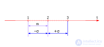
Studying the law, we can determine that: m x = 1 / λ , σ = 1 / λ , that is, for the simplest flow, m x = σ . The equality of expectation to the standard deviation means that this flow is a flow without an after-effect. The variance (more precisely, the standard deviation) of such a flow is large. Physically, this means that the time of occurrence of an event (distance between events) is poorly predictable, accidentally, is in the interval m x - σ < τ j < m x + σ . Although it is clear that on average it is approximately equal: τ j = m x = T n / N. An event may occur at any time, but within the range of this moment τ j with respect to m x on [- σ ; + σ ] (magnitude of the aftereffect). In fig. 28.5 shows the possible positions of event 2 relative to the time axis for a given σ . In this case, they say that the first event does not affect the second, the second to the third, and so on, that is, there is no response.
|
|
| Fig. 28.5. Illustration of the effect of σ position of the event on the timeline |
In the sense of P, it is equal to r (see Lecture 23. Modeling a random event. Modeling the full group of incompatible events), therefore, expressing τ from the formula (*) , finally, to determine the intervals between two random events, we have:
τ = –1 / λ · Ln ( r ) ,
where r is a random number uniformly distributed from 0 to 1, which is taken from the RNG, τ is the interval between random events (random variable τ j ).
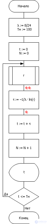
Example 1. Consider the flow of products arriving at a process operation. Products come randomly - an average of eight pieces per day (flow intensity λ = 8/24 [units / hour]). It is necessary to simulate this process for T n = 100 hours. m = 1 / λ = 24/8 = 3, that is, on average, one part in three hours. Note that σ = 3. In fig. 28.6 presents an algorithm that generates a stream of random events.
|
|
| Fig. 28.6. Algorithm generating thread random events in given λ |
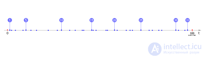
In fig. 28.7 shows the result of the algorithm - the points in time when the details came to the operation. As can be seen, in just the period T n = 100, the production unit processed N = 33 products. If the algorithm is run again, then N can be equal, for example, 34, 35 or 32. But on average, for K runs of algorithm N will be 33.33 ... If you count the distances between events t with i and the moments of time defined as 3 · i , then the average value will be equal to σ = 3.
|
|
| Fig. 28.7. Illustration of the algorithm that generates a stream of random events |
If it is known that the flow is not ordinary, then it is necessary to model in addition to the moment of the occurrence of the event also the number of events that could appear at that moment. For example, cars to a railway station arrive as part of a train at random times (ordinary train flow). But at the same time, the train may have a different (random) number of cars. In this case, the flow of cars is referred to as a stream of unusual events.
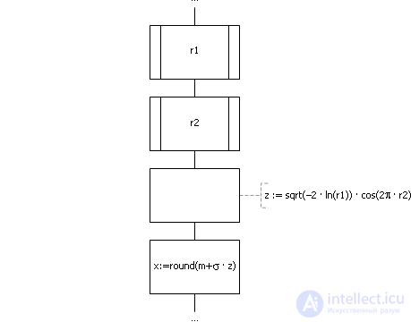
Suppose that M k = 10, σ = 4 (that is, on average in 68 cases from 6 to 14 wagons are included in the train) and their number is distributed according to the normal law. In the place marked with (*) in the previous algorithm (see Fig. 28.6), you need to insert the fragment shown in Fig. 28.8.
|
|
| Fig. 28.8. A fragment of the algorithm that implements extraordinary flow of random events |
Example 2. The following task is very useful in production. What is the average daily idle time of a technological node, if a node processes each item at a random time given by the intensity of the random event flow λ 2 ? At the same time, it was established experimentally that products are also brought for processing at random times given by a stream of λ 1 in batches of 8 pieces, and the lot size varies randomly according to the normal law with m = 8, σ = 2 (see Chapter 25). Before the start of the simulation, T = 0, there were no products in stock. It is necessary to simulate this process for T n = 100 hours.
In fig. Figure 28.9 shows an algorithm that randomly generates a flow of arrivals of batches of products for processing and a stream of random events — the exit of batches of products from processing.
|
|
| Fig. 28.9. Algorithm imitation processing batches of products taking into account the randomness of the events |
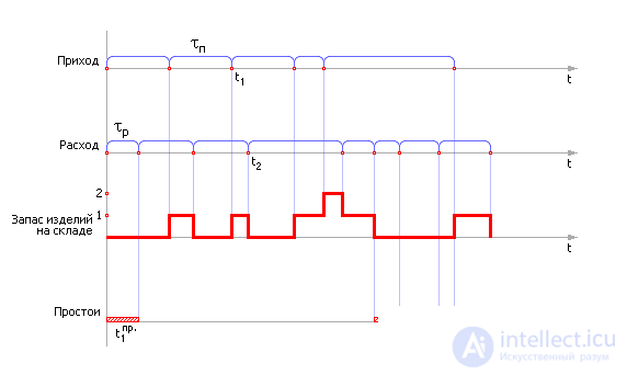
In fig. 28.10 shows the result of the algorithm - the moments of time when the parts arrived at the operation, and the moments of time when the parts left the operation. On the third line you can see how many parts were queuing for processing (lay at the node warehouse) at different points in time.
|
|
| Fig. 28.10. Diagram illustrating the movement of products through the processing unit |
Noting the times for the processing node when it was idle waiting for the next part (see Fig. 28.10 for the time allotted in red hatching), we can calculate the total node downtime during the entire observation time, and then calculate the average downtime during the day. For this implementation, this time is calculated as:
T av. Wed = 24 · ( t 1 ave. + T 2 ave. + T 3 ave. + T 4 ave. +… + T N ave. ) / T n .
Task 1. Changing the value of σ , set the dependence T Ave. cf. ( σ ). Setting the cost for a simple node of 100 euros / hour, set the annual loss of the company from irregularity in the work of suppliers. Offer the wording of the clause of the contract of the enterprise with the suppliers “The amount of the penalty for the delay in the delivery of products”.
Task 2. Changing the value of the initial filling of the warehouse, set how the annual losses of the enterprise from the irregularity in the work of the suppliers will change depending on the size of the stocks accepted at the enterprise.
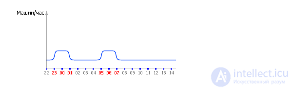
In some cases, the flux intensity may vary with time λ ( t ). Such a flow is called stationary. For example, the average number per hour of ambulance cars leaving the station at the calls of the population of a large city may vary during the day. It is known, for example, that the greatest number of calls falls at intervals from 23 to 01 in the morning and from 05 to 07 in the morning, whereas in the rest of the hours it is half as much (see Fig. 28.11).
|
|
| Fig. 28.11. Chart of change of intensity of a stream of random events with time |
In this case, the distribution of λ ( t ) can be specified either by a graph, or by a formula, or by a table. And in the algorithm shown in fig. 28.6, in the place marked (**), it will be necessary to insert the fragment shown in fig. 28.12.
|
|
| Fig. 28.12. Fragment of the algorithm that implements the generation random events in case of unsteady flow |


Comments
To leave a comment
System modeling
Terms: System modeling