Lecture
If an object is characterized by a certain parameter that is different in its value at different points of the object, then we can say that the values of such a parameter are distributed (over the object). If there are several such parameters, then the object is considered as a system with distributed parameters. In order to make calculations, it is convenient to divide the system into elementary volumes (layers). Let's show it by example.
Example 1. Consider the process of drying the material (see fig. 17.1). Assume that the material is a pile of raw materials over which a heater is installed. In the process of drying, heat unevenly penetrates deep into the heap, and in different layers the material has a different temperature. That is, in this example, we can say that the temperature parameter is distributed over the “heap” object. We describe each layer by our equation using the procedure for constructing a model for a separate layer from lecture 11.
|
|
| Fig. 17.1. Process flow diagram drying the material broken into layers |
The temperature change in the first layer (T n - heater temperature, T cf - medium temperature):

Temperature change in the i-th layer:
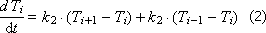
Temperature change in the nth layer:
Then the behavior of the system “heaps of raw materials” is described by a system of differential equations , each of which describes a separate layer of “heaps”.
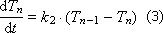
The algorithm for calculating such a system is shown in Fig. 17.2. A feature of the algorithm is that it contains, in addition to the cycle in time (see the algorithm in Fig. 10.5), the nested loop by layer number. Indeed, on each measure, it is necessary to separately calculate the changes in each of the heap layers. The distribution of the object (the introduction of an additional coordinate) is simulated by an additional cyclic block .
|
|
| Fig. 17.2. Flowchart simulation of distributed systems (for example, the drying process) |
Again, attention should be paid to the fact that the cycle for calculating derivatives and the cycle for calculating the new state of the system are separated from each other in order to avoid the appearance of a “race effect”.
So, the tool for modeling distributed systems is nested loops , at least double ones - inside the loop “in time” there is a loop “in space”.
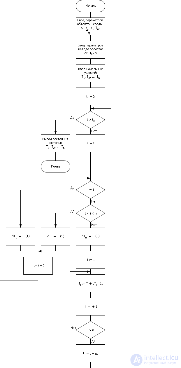
The model may look different - depending on the platform on which it is implemented. Above (see Fig. 17.2), an example was analyzed showing the algorithmic method of describing the calculation of the behavior of a distributed system using the background language and architecture of the Neumann machine (see Fig. 17.3).
|
|
| Fig. 17.3. Background Neumann computing system architecture (with a common bus, a star) |
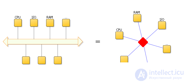
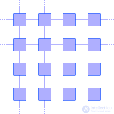
Imagine that we are using for modeling the structure of a non-background Neumann machine (see lecture 02 of the AI), which consists of a MULTIPLE of elementary identical computing elements interconnected in a network (see. Fig. 17.4). With this architecture, the elements exist simultaneously, that is, parallel synchronously in time and at the end of each clock cycle, output (input) signals are exchanged between themselves and their neighbors in the network. Such a computing platform paradigm imitates the world around us more adequately.
|
|
| Fig. 17.4. Not a background Neumann architecture computing system (homogeneous, parallel network of computing elements) |
Using the von Neumann machine, architecture with a common bus (star), we thereby organize the computational process algorithmically, representing it as a sequence of steps. The algorithm itself is performed on the same resource - the only processor that, through the bus (the star's central node), requests, step by step, the memory about the state of each of the elements it calculates. The central node (bus) is thus a bottleneck. The processor processes tact by cycle for each element of the simulated system, which are lined up for processing.
In the world around us, which we are trying to imitate, in fact, entities are autonomous, they live as if parallel to themselves in time, manifesting their properties through interaction with their neighbors in space.
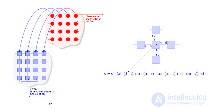
Let us put in one-to-one correspondence elementary entities of a simulated complex object from the real world to elementary calculators - each computational element will imitate one specific entity (see. Fig. 17.5, a). To do this, in the computational element, we write down the law of the functioning of exactly the entity that it will imitate (see Fig. 17.5, b).
|
|
| Fig. 17.5. Illustration of the principle of object reflection of the world in information models |
For our problem of calculating thermal conductivity, the record of the law of temperature change for an elementary volume will be as follows:
s: = s + (al · (sl - s) + ar · (sr - s) + au · (su - s) + ab · (sn - s)) · dt.
Each element of the computer network performs the same, and, unique, operation, implements the same model, and, moreover, elementary. This is a feature of parallel structures.
Next, we will connect the computational elements with connections in the same way as the elements of the real world are in contact with each other.
Then the element will transfer information about its temperature s to the left element in its variable sr, the right element in its variable sl, the top element in its variable sb, the lower element from it in its variable st (see fig. 17.5, b) . at, ar, al, ab are the coefficients of thermal conductivity in the corresponding directions. The variable s is changed by the value of the heat fluxes suitable from these directions per time step dt: s: = s + (...) · dt. Having established, thus, the connections of all elements, we obtain a similarity of a computer network to a real distributed object.
Pay attention, the algorithm shown by us on fig. 17.2, disappears, giving way to a model. In the model entry, nothing reminds us of the specifics of the implementation environment. There are no algorithmic structures, respectively, and there is no need for constructions that are extraneous with respect to the object being simulated (if, while, etc.). This is due to the fact that we use a more complete similarity of the simulated system to the platform on which its simulation is performed. When using the von Neumann structure, we are forced to make a special additional translation from the object language to the machine language (algorithmization procedure), which is not related to the real object, but related to the implementation environment. Therefore, one should try to pay attention to the ADEQUACY of the platform (architecture, description language) on which the modeling is performed, to the real structure of the world around us. Try to establish the greatest LIKE between them at the stage of development.
So, there are two fundamentally different computational architectures — the Neumann background and the non-Neumann background (both proposed by von Neumann):
Example. We simulate the thermal conductivity of a house of two rooms interconnected by doors. In the system we take into account the possibility of communicating rooms with the environment through the windows and the front door.
Launch three projects in succession: House-1, House-2 and House-3.
Please note, in the first case, we consider the room as one. The house is a concentrated system of two elements, on which the environment acts  and additional (external) heat sources (batteries)
  . In this case, the project developer assumes the temperature in different places of one single room.
In model 2, the designer complicated the project by installing additional interface components into it for ease of use. We see the process of formalization in development. An interface is superimposed on the model, the important thing here is that it is separated from the model in this notation. We can easily replace individual interface elements independently of each other.
If we want to clarify the model, assuming that the temperatures in different corners of the room may be different , which is actually the case, then we will have to divide the rooms into smaller elements , organize their description and establish connections between them. Imitation will become more accurate, so in model 3 you can already explore more subtle effects - try opening and closing windows and doors, changing the temperatures of heating devices and the environment and look at the result (see Fig. 17.6).
|
|
| Fig. 17.6. Result of the work of the distributed system model under various conditions and external influences |
Note. In fairness, it should be noted that, despite the fact that you see elements of the computer network, you end up imitating a serial machine (a process machine, an algorithmic machine) for lack of currently you do not have a background Neumann machine. Compensates (masks) the complexity of the algorithmic way of thinking modeling environment Stratum-2000, which simulates the work of a parallel object-oriented machine on the background Neumann structure. But if you didn’t have the background of the Neumann machine, you would automatically transfer the project to the computer network without any changes. Such a transfer is called the reflection of the object in the simulation environment.
That is, in draft 3, we actually see a parallel object-oriented system. The structure is not the background of the Neumann machine supports an object-oriented modeling method (see Lecture 32).


Comments
To leave a comment
System modeling
Terms: System modeling