Simulation of a random variable system

Often in practice there are systems of random variables, that is, such two (and more) different random variables X , Y (and others) that depend on each other. For example, if an event X occurred and took some random value, then the Y event occurs, although by chance, but taking into account that X has already taken some meaning.

For example, if a large number falls out as X , then Y should fall out also a sufficiently large number (if the correlation is positive). It is very likely that if a person has a lot of weight, then he will most likely be of great height. Although this is NOT MANDATORY, it is NOT the REGULARITY, but the correlation of random variables. Since there are, albeit rarely, people with a large weight, but of small stature or with a small weight and high. And yet, the majority of obese people are high, and low people have low weight.

By definition, if the random variables are independent, then f ( x ) = f ( x ₁ ) · f ( x ₂ ) ·… · f ( x _n ).

If the random variables are dependent, then f ( x ) = f ( x ₁ ) · f ( x ₂ | x ₁ ) · f ( x ₃ | x ₂ , x ₁ ) · ... · f ( x _n | x _{n - 1} , x _{n - 2} , ..., x ₂ , x ₁ ).

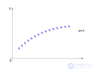
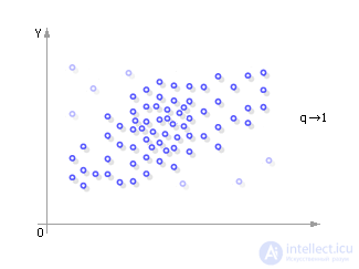
Let, for example, there are two dependent events - X and Y , distributed according to the normal law. X has a mean of m _x and a standard deviation of σ _x . Y has a mean of m _y and a standard deviation σ _y . The correlation coefficient - q - shows how closely the events X and Y are related. If the correlation coefficient is equal to one, then the dependence of the events X and Y is one-to-one: one value of X corresponds to one value of Y (see fig. 26.1).

Fig. 26.1. Type of dependence of two random variables with a positive correlation coefficient (q = 1)

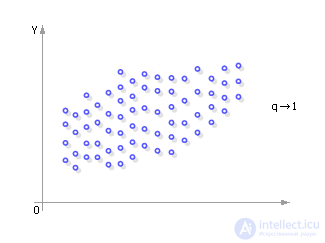
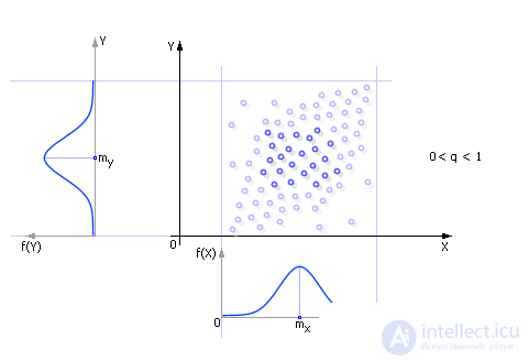
When q is close to unity, the picture shown in fig. 26.2, that is, several Y values ​​(more precisely, one of several Y values ​​randomly determined) may correspond to one X value; in this case, X and Y events are less correlated, less dependent on each other.

Fig. 26.2. Type of dependence of two random variables with a positive correlation coefficient (0 <q <1)

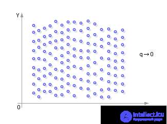
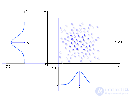
And finally, when the correlation coefficient tends to zero, a situation arises in which any value of X can correspond to any value of Y , that is, events X and Y do not depend on or almost do not depend on each other, do not correlate with each other (see Figure 26.3).

Fig. 26.3. Type of dependence of two random variables with a correlation coefficient close to zero (q -> 0)

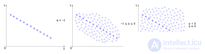
On all graphs, the correlation was taken as a positive value. If q <0, then the graphs will look like the one shown in fig. 26.4.

Fig. 26.4. Type of dependence of two random variables with a negative correlation coefficient a) q = –1; b) –1 <q <0; c) q -> 0

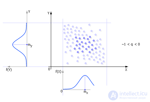
In fact, random events ( X and Y ) cannot take any values ​​with equal probability, as is the case in Fig. 26.2. For example, in a group of students there cannot be people of super-small or extra-large growth; Mostly, people have a certain average growth and variation around this average growth. Therefore, on some parts of the X axis the number of events is located more densely, on others - less often. (The density of random events, the number of points on the graphs is greater near the values ​​of m _x ). The same is true for Y. And then rice. 26.2 can be depicted more accurately, as shown in Fig. 26.5.

Fig. 26.5. Illustration of a system of random dependent variables

For example, take the normal distribution, as the most common. The expectation indicates the most probable events, here the number of events is greater and the schedule of events is thicker. A positive correlation indicates (see Fig. 26.2) that large random variables X cause large Y to be generated. A negative correlation indicates (see Fig. 26.4) that large random variables X stimulate to generate smaller random variables Y. The zero and close to zero correlation shows (see Fig. 26.3) that the magnitude of the random variable X is in no way connected with a certain value of the random variable Y. It is easy to understand what has been said if we first imagine the distributions of f ( X ) and f ( Y ) separately, and then link them into the system (see Fig. 26.6, Fig. 26.7 and Iris. 26.8).

Fig. 26.6. Random System Generation with a positive correlation coefficient

Fig. 26.7. Random System Generation with a negative correlation coefficient

Fig. 26.8.

An example of the implementation of the algorithm for modeling two dependent random events X and Y. Condition: Assume that X and Y are distributed according to the normal law with the corresponding values m _x , σ _x and m _y , σ _y . Given the correlation coefficient of two random events q , that is, the random variables X and Y are dependent on each other, Y is not entirely random.

Then the possible algorithm for implementing the model will be as follows.

1. Playing six random evenly distributed on the interval [0; 1] numbers b ₁ , b ₂ , b ₃ , b ₄ , b ₅ , b ₆ ; their sum is S : S = b ₁ + b ₂ + b ₃ + b ₄ + b ₅ + b ₆ . The normally distributed random number x is found according to the following formula: x = sqrt (2) · σ _x · ( S - 3) + m _x , see division 25.
2. By the formula m _{y / x} = m _y + q · σ _y / σ _x · ( x - m _x ) the expectation m _{y / x is found} (the sign y / x means that y will take random values ​​taking into account the condition that x already adopted some specific values).
3. By the formula σ _{y / x} = σ _y · sqrt (1 - q ² ) the standard deviation σ _{y / x is found} (the sign y / x means that y will take random values ​​taking into account the condition that x has already taken some specific values ).
4. Playing six random evenly distributed on the interval [0; 1] numbers r ₁ , r ₂ , r ₃ , r ₄ , r ₅ , r ₆ ; their sum k is found : k = r ₁ + r ₂ + r ₃ + r ₄ + r ₅ + r ₆ . The normally distributed random number y is found using the following formula: y = sqrt (2) · σ _{y / x} · ( k - 3) + m _{y / x} .