Linear regression models

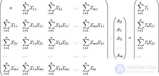
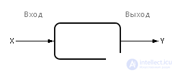
For research purposes, it is often convenient to present the object under study in the form of a box that has entrances and exits, without considering in detail its internal structure. Of course, the transformations in the box (on the object) occur (the signals travel through connections and elements, change their shape, etc.), but with such a view they occur hidden from the observer.

According to the degree of awareness of the researcher about the object, there is a division of objects into three types of "boxes":

• “White box”: everything is known about the object;
• “Gray box”: the structure of the object is known, the quantitative values ​​of the parameters are unknown;
• “Black box”: nothing is known about the object.

The black box is conventionally depicted as in fig. 2.1.

Fig. 2.1. Black box designation on diagrams

The values ​​at the inputs and outputs of the black box can be monitored and measured. The contents of the box is unknown.

The task is to, knowing the set of values ​​at the inputs and outputs, to build a model, that is, to determine the function of the box, according to which the input is converted to output. Such a task is called a regression analysis problem.

Depending on whether the inputs are available to the investigator for control or only for observation, one can speak of an active or passive experiment with the box.

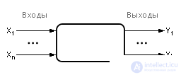
Let, for example, we face the task of determining how the output of products depends on the amount of electricity consumed. The results of the observations will be displayed on the graph (see figure 2.2). There are a total of n experimental points on the graph, which correspond to n observations.

Fig. 2.2. Graphic view of the results black box observation

To begin with, suppose we are dealing with a black box that has one entrance and one exit. Suppose for simplicity that the relationship between input and output is linear or nearly linear. Then this model will be called a linear one-dimensional regression model.

1) The researcher makes a hypothesis about the structure of the box

Considering the experimentally obtained data, suppose that they obey the linear hypothesis, that is, the output Y depends on the input X linearly, that is, the hypothesis has the form: Y = A ₁ X + A ₀ (Fig. 2.2).

2) Determination of unknown coefficients A ₀ and A ₁ models

Linear one-dimensional model (Fig. 2.3).

Fig. 2.3. One-dimensional black box model

For each of the n experimentally taken points, we calculate the error ( E _i ) between the experimental value ( Y _i ^Exp. ) And the theoretical value ( Y _i ^Th. ), Which lies on the hypothetical straight line A ₁ X + A ₀ (see Fig. 2.2):

E _i = ( Y _i ^Exp. - Y _i ^Theor. ), I = 1, ..., n ;

E _i = Y _i - A ₀ - A ₁ · X _i , i = 1, ..., n .

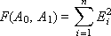
Errors E _i for all n points should be added. So that the positive errors do not compensate for the negative in total, each of the errors is squared and their values ​​are added to the total error F of the same sign:

E _i ² = ( Y _i - A ₀ - A ₁ · X _i ) ² , i = 1, ..., n .

The purpose of the method is to minimize the total error F due to the selection of the coefficients A ₀ , A ₁ . In other words, this means that it is necessary to find such coefficients A ₀ , A _{1 of the} linear function Y = A ₁ X + A ₀ so that its graph runs as close as possible simultaneously to all experimental points. Therefore, this method is called the method of least squares.

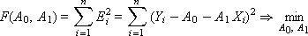
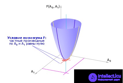
The total error F is a function of two variables A ₀ and A ₁ , that is, F ( A ₀ , A ₁ ), by changing which, it is possible to influence the magnitude of the total error (see Fig. 2.4).

Fig. 2.4. Approximate view of the error function

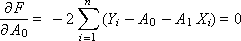
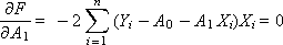
To minimize the total error, we find the partial derivatives of the function F for each variable and equate them to zero (the extremum condition):

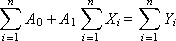
After opening the brackets, we obtain a system of two linear equations:

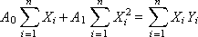
To find the coefficients A ₀ and A ₁ by the Kramer method, we represent the system in matrix form:

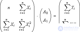
The solution is:

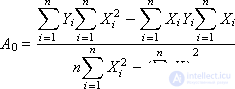
Calculate the values ​​of A ₀ and A ₁ .

3) Verification

To determine whether a hypothesis is accepted or not, it is necessary, first, to calculate the error between the points of the given experimental and theoretical dependencies obtained and the total error:

E _i = ( Y _i ^Exp. - Y _i ^Theor. ), I = 1, ..., n

And, secondly, it is necessary to find the value of σ by the formula , where F is the total error, n is the total number of experimental points.

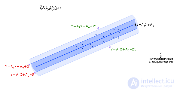
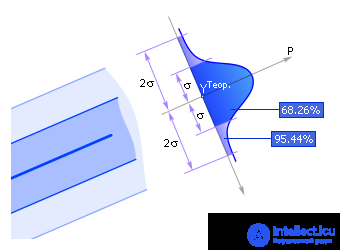
If in a strip bounded by lines Y ^Theor. - S and Y ^Theor. + S (Fig. 2.5), falls 68.26% or more of the experimental points Y _i ^Exp. then the hypothesis put forward by us is accepted. Otherwise, choose a more complex hypothesis or check the source data. If greater confidence is required in the result, then an additional condition is used: in the band bounded by the Y ^Theor lines ^. - 2 S and Y ^Theor. + 2 S , should fall 95.44% or more of the experimental points Y _i ^Exp. .

Fig. 2.5. Study of the acceptability of accepting a hypothesis

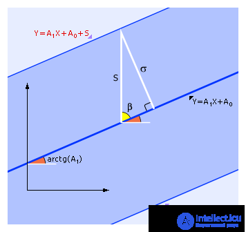
The distance S is related to σ as follows:

S = σ / sin ( β ) = σ / sin (90 ° - arctan ( A ₁ )) = σ / cos (arctan ( A ₁ )),

which is illustrated in fig. 2.6.

Fig. 2.6. The relationship of the values ​​of σ and S

The condition for accepting a hypothesis is derived from the normal distribution of random errors (see Fig. 2.7). P is the probability distribution of the normal error.

Fig. 2.7. Law illustration normal error distribution

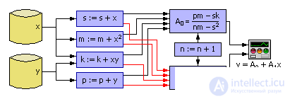
Finally, we give in fig. 2.8 graphical scheme of the implementation of a one-dimensional linear regression model

Fig. 2.8. Method implementation scheme least squares in the simulation environment

Practice # 01: Regression Models

Lab №01: "Linear regression models"

Linear multiple model

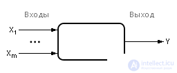
Suppose that the functional structure of the box again has a linear relationship, but the number of input signals acting simultaneously on an object is m (see Fig. 2.9):

Y = A ₀ + A ₁ · X ₁ +… + A _m · X _m .

Fig. 2.9. Designation of multidimensional black box diagrams

Since it is assumed that we have experimental data on all inputs and outputs of the black box, we can calculate the error between the experimental ( Y _i ^Exp. ) And theoretical ( Y _i ^Theor. ) Y value for each i -th point (albeit before, the number of experimental points is n ):

E _i = ( Y _i ^Exp. - Y _i ^Theor. ), I = 1, ..., n ;

E _i = Y _i - A ₀ - A ₁ · X _{1 i} - ... - A _m · X _mi , i = 1, ..., n .

Minimize the total error F :

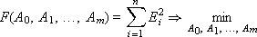
Error F depends on the choice of the parameters A ₀ , A ₁ , ..., A _m . To find the extremum, we equate all partial derivatives of F over unknowns A ₀ , A ₁ , ..., A _m to zero:

We obtain a system of m + 1 equations with m + 1 unknowns, which should be solved in order to determine the coefficients of the linear multiple model A ₀ , A ₁ , ..., A _m . To find the coefficients by the Kramer method, we present the system in a matrix form:

We calculate the coefficients A ₀ , A ₁ , ..., A _m .

Further, by analogy with the one-dimensional model (see 3). “Check”), for each point the error E _{i is} calculated; then, the total error F and the values ​​of σ and S are found to determine whether the advanced hypothesis about the linear multidimensional black box is accepted or not.

With the help of substitutions and redefinitions to the linear multiple model, many nonlinear models are given. Details about this are described in the material of the next lecture.