Lecture
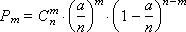
The most common case of various kinds of probability distributions is the binomial distribution. We will use its universality to determine the most common in practice particular types of distributions.
Suppose there is some event A. The probability of occurrence of event A is equal to p , the probability of non-occurrence of event A is 1 - p , sometimes it is designated as q . Let n be the number of trials, m be the frequency of occurrence of event A in these n trials.
It is known that the total probability of all possible combinations of outcomes is equal to one, that is:
1 = p n + n · p n - 1 · (1 - p ) + C n n - 2 · p n - 2 · (1 - p ) 2 +… + C n m · p m · (1 - p ) n - m + ... + (1 - p ) n .
|
The expectation M of the binomial distribution is:
M = n · p ,
where n is the number of tests, p is the probability of an event A.
Standard deviation σ :
σ = sqrt ( n · p · (1 - p )).
Example 1. Calculate the probability that an event that has a probability p = 0.5 will occur m = 1 times in n = 10 trials. We have: C 10 1 = 10, and further: P 1 = 10 · 0.5 1 · (1 - 0.5) 10 - 1 = 10 · 0.5 10 = 0.0098. As you can see, the probability of occurrence of this event is quite small. This is explained, firstly, by the fact that it is absolutely not clear whether an event will occur or not, since the probability is 0.5 and the odds here are “50 to 50”; and secondly, it is required to calculate that the event will occur exactly once (no more and no less) out of ten.
Example 2. Calculate the probability that an event that has a probability p = 0.5 in m = 10 trials will occur m = 2 times. We have: C 10 2 = 45, and further: P 2 = 45 · 0.5 2 · (1 - 0.5) 10 - 2 = 45 · 0.5 10 = 0.044. The likelihood of this event has become more!
Example 3. Increase the likelihood of the event itself. Let's make it more likely. Calculate the probability that an event that has a probability p = 0.8, in n = 10 trials will occur m = 1 times. We have: C 10 1 = 10, and further: P 1 = 10 · 0.8 1 · (1 - 0.8) 10 - 1 = 10 · 0.8 1 · 0.2 9 = 0.000004. The probability has become less than in the first example! The answer, at first glance, seems strange, but since the event has a sufficiently high probability, it is unlikely that it will occur only once. It is more likely that it will happen more than once, the number of times. Indeed, counting P 0 , P 1 , P 2 , P 3 , ..., P 10 (the probability that an event in the n = 10 trials will occur 0, 1, 2, 3, ..., 10 times), we will see:
C 10 0 = 1, C 10 1 = 10, C 10 2 = 45, C 10 3 = 120, C 10 4 = 210, C 10 5 = 252,
C 10 6 = 210, C 10 7 = 120, C 10 8 = 45, C 10 9 = 10, C 10 10 = 1;
P 0 = 1 · 0.8 0 · (1 - 0.8) 10 - 0 = 1 · 1 · 0.2 10 = 0.0000…;
P 1 = 10 · 0.8 1 · (1 - 0.8) 10 - 1 = 10 · 0.8 1 · 0.2 9 = 0.0000…;
P 2 = 45 · 0.8 2 · (1 - 0.8) 10 - 2 = 45 · 0.8 2 · 0.2 8 = 0.0000…;
P 3 = 120 · 0.8 3 · (1 - 0.8) 10 - 3 = 120 · 0.8 3 · 0.2 7 = 0.0008 ...;
P 4 = 210 · 0.8 4 · (1 - 0.8) 10 - 4 = 210 · 0.8 4 · 0.2 6 = 0.0055 ...;
P 5 = 252 · 0.8 5 · (1 - 0.8) 10 - 5 = 252 · 0.8 5 · 0.2 5 = 0.0264 ...;
P 6 = 210 · 0.8 6 · (1 - 0.8) 10 - 6 = 210 · 0.8 6 · 0.2 4 = 0.0881 ...;
P 7 = 120 · 0.8 7 · (1 - 0.8) 10 - 7 = 120 · 0.8 7 · 0.2 3 = 0.2013 ...;
P 8 = 45 · 0.8 8 · (1 - 0.8) 10 - 8 = 45 · 0.8 8 · 0.2 2 = 0.3020 ... (the highest probability!);
P 9 = 10 · 0.8 9 · (1 - 0.8) 10 - 9 = 10 · 0.8 9 · 0.2 1 = 0.2684…;
P 10 = 1 · 0.8 10 · (1 - 0.8) 10 - 10 = 1 · 0.8 10 · 0.2 0 = 0.1074 ...
Of course, P 0 + P 1 + P 2 + P 3 + P 4 + P 5 + P 6 + P 7 + P 8 + P 9 + P 10 = 1.
If we depict the values of P 0 , P 1 , P 2 , P 3 , ..., P 10 , which we calculated in example 3, on the graph, it turns out that their distribution has a form close to the normal distribution law (see. Fig. 27.1 ) (see lecture 25. Modeling normally distributed random variables).
| |
| Fig. 27.1. Type of binomial distribution probabilities for different m at p = 0.8, n = 10 |
The binomial law goes over to normal, if the probabilities of occurrence and non-occurrence of event A are about the same, that is, we can conditionally write: p ≈ (1 - p ). For example, take n = 10 and p = 0.5 (that is, p = 1 - p = 0.5).
We will come to this task meaningfully, for example, if we want to theoretically calculate how many boys there will be and how many girls out of 10 children born at the maternity hospital in one day. More precisely, we will consider not boys and girls, but the probability that only boys will be born, that 1 boy and 9 girls will be born, that 2 boys and 8 girls will be born, and so on. Let us assume for simplicity that the probability of having a boy and a girl is the same and equal to 0.5 (but in fact, to be honest, this is not the case, see the course “Modeling artificial intelligence systems”).
It is clear that the distribution will be symmetrical, since the probability of having 3 boys and 7 girls is equal to the probability of having 7 boys and 3 girls. The highest probability of birth will be in 5 boys and 5 girls. This probability is equal to 0.25, by the way, it is not so great in absolute value. Further, the probability that 10 or 9 boys will be born at once is much less than the probability that 5 ± 1 boys from 10 children will be born. Just the binomial distribution will help us to make this calculation. So.
C 10 0 = 1, C 10 1 = 10, C 10 2 = 45, C 10 3 = 120, C 10 4 = 210, C 10 5 = 252,
C 10 6 = 210, C 10 7 = 120, C 10 8 = 45, C 10 9 = 10, C 10 10 = 1;
P 0 = 1 · 0.5 0 · (1 - 0.5) 10 - 0 = 1 · 1 · 0.5 10 = 0.000977 ...;
P 1 = 10 · 0.5 1 · (1 - 0.5) 10 - 1 = 10 · 0.5 10 = 0.009766 ...;
P 2 = 45 · 0.5 2 · (1 - 0.5) 10 - 2 = 45 · 0.5 10 = 0.043945…;
P 3 = 120 · 0.5 3 · (1 - 0.5) 10 - 3 = 120 · 0.5 10 = 0.117188…;
P 4 = 210 · 0.5 4 · (1 - 0.5) 10 - 4 = 210 · 0.5 10 = 0.205078 ...;
P 5 = 252 · 0.5 5 · (1 - 0.5) 10 - 5 = 252 · 0.5 10 = 0.246094…;
P 6 = 210 · 0.5 6 · (1 - 0.5) 10 - 6 = 210 · 0.5 10 = 0.205078 ...;
P 7 = 120 · 0.5 7 · (1 - 0.5) 10 - 7 = 120 · 0.5 10 = 0.117188…;
P 8 = 45 · 0.5 8 · (1 - 0.5) 10 - 8 = 45 · 0.5 10 = 0.043945…;
P 9 = 10 · 0.5 9 · (1 - 0.5) 10 - 9 = 10 · 0.5 10 = 0.009766 ...;
P 10 = 1 · 0.5 10 · (1 - 0.5) 10 - 10 = 1 · 0.5 10 = 0.000977 ...
Of course, P 0 + P 1 + P 2 + P 3 + P 4 + P 5 + P 6 + P 7 + P 8 + P 9 + P 10 = 1.
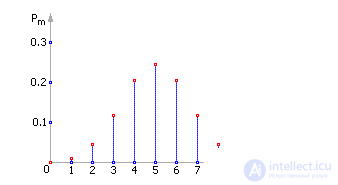
Let's reflect on the graph the values of P 0 , P 1 , P 2 , P 3 , ..., P 10 (see. Fig. 27.2).
| |
| Fig. 27.2. Graph of the binomial distribution with parameters p = 0.5 and n = 10, bringing it closer to the normal law |
So, under the conditions m ≈ n / 2 and p ≈ 1 - p or p ≈ 0.5, the normal distribution can be used instead of the binomial distribution. For large values of n, the graph shifts to the right and becomes more and more flat as the mean and variance increase with increasing n : M = n · p , D = n · p · (1 - p ).
By the way, the binomial law tends to normal and with increasing n , which is quite natural, according to the central limit theorem (see Lecture 34. Fixing and processing statistical results).
Now let us consider how the binomial law changes in the case when p ≠ q , that is, p -> 0. In this case, the hypothesis on the normality of the distribution cannot be applied, and the binomial distribution goes into the Poisson distribution.
The Poisson distribution is a special case of the binomial distribution (with n >> 0 and with p -> 0 (rare events)).
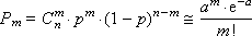
A formula is known from mathematics that makes it possible to approximately calculate the value of any member of the binomial distribution:

where a = n · p is the Poisson parameter (mathematical expectation), and the variance is equal to the mathematical expectation. We present the mathematical calculations explaining this transition. Binomial distribution law
P m = C n m · p m · (1 - p ) n - m
can be written, if we put p = a / n , in the form
or

Since p is very small, only numbers m should be taken into account, small in comparison with n . Composition
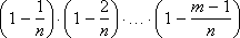
very close to one. The same applies to the value

Magnitude

very close to e - a . From here we get the formula:
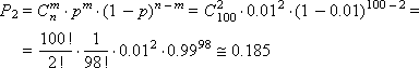
Example. The box contains n = 100 parts, both quality and defective. The probability of getting a defective product is p = 0.01. Suppose that we remove the product, determine whether it is defective or not, and put it back. Acting in this way, it turned out that out of 100 products that we reviewed, two turned out to be defective. What is the probability of this?
By the binomial distribution we get:
By the Poisson distribution we get:

As can be seen, the values turned out to be close, therefore, in the case of rare events, it is completely permissible to apply the Poisson law, especially since it requires less computational costs.
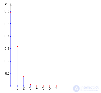
Let us graphically show the Poisson law. Take for example the parameters p = 0.05, n = 10. Then:
C 10 0 = 1, C 10 1 = 10, C 10 2 = 45, C 10 3 = 120, C 10 4 = 210, C 10 5 = 252,
C 10 6 = 210, C 10 7 = 120, C 10 8 = 45, C 10 9 = 10, C 10 10 = 1;
P 0 = 1 · 0.05 0 · (1 - 0.05) 10 - 0 = 1 · 1 · 0.95 10 = 0.5987 ...;
P 1 = 10 · 0.05 1 · (1 - 0.05) 10 - 1 = 10 · 0.05 1 · 0.95 9 = 0.3151 ...;
P 2 = 45 · 0.05 2 · (1 - 0.05) 10 - 2 = 45 · 0.05 2 · 0.95 8 = 0.0746 ...;
P 3 = 120 · 0.05 3 · (1 - 0.05) 10 - 3 = 120 · 0.05 3 · 0.95 7 = 0.0105 ...;
P 4 = 210 · 0.05 4 · (1 - 0.05) 10 - 4 = 210 · 0.05 4 · 0.95 6 = 0.00096 ...;
P 5 = 252 · 0.05 5 · (1 - 0.05) 10 - 5 = 252 · 0.05 5 · 0.95 5 = 0.00006 ...;
P 6 = 210 · 0.05 6 · (1 - 0.05) 10 - 6 = 210 · 0.05 6 · 0.95 4 = 0.0000 ...;
P 7 = 120 · 0.05 7 · (1 - 0.05) 10 - 7 = 120 · 0.05 7 · 0.95 3 = 0.0000 ...;
P 8 = 45 · 0.05 8 · (1 - 0.05) 10 - 8 = 45 · 0.05 8 · 0.95 2 = 0.0000 ...;
P 9 = 10 · 0.05 9 · (1 - 0.05) 10 - 9 = 10 · 0.05 9 · 0.95 1 = 0.0000 ...;
P 10 = 1 · 0.05 10 · (1 - 0.05) 10 - 10 = 1 · 0.05 10 · 0.95 0 = 0.0000 ...
Of course, P 0 + P 1 + P 2 + P 3 + P 4 + P 5 + P 6 + P 7 + P 8 + P 9 + P 10 = 1.
| |
| Fig. 27.3. Poisson distribution graph for p = 0.05 and n = 10 |
When n -> ∞, the Poisson distribution goes over to the normal law, according to the central limit theorem (see Lecture 34. Fixing and processing statistical results).
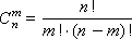 - the number of combinations of n by m .

Comments
To leave a comment
System modeling
Terms: System modeling