Lecture
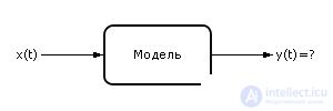
Let us know the input dynamic sequence X (input signal) and the model (method of converting the input signal into the output signal). The problem of determining the output signal y ( t ) is being considered (see Fig. 10.1).
|
|
| Fig. 10.1. Structural model of a dynamic system with one entrance and one exit |
A model of a dynamic system can be represented by a differential equation. The basic equation of dynamics:
y ' = f ( x ( t ), y ( t ), t ).
The initial conditions at the zero moment of time t 0 : y ( t 0 ), x ( t 0 ) are known. To determine the output signal, note that, by definition, the derivative:
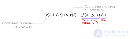
We know the position of the system at the point "1", it is required to determine the position of the system at the point "2". The points are separated from each other by the distance Δ t (Fig. 10.2). That is, the calculation of the behavior of the system is made in steps. From point “1” we jump (discretely) to point “2”, the distance between points along the axis t is called the calculation step Δ t .
|
|
| Fig. 10.2. Illustration of the calculation of the future state of the system Euler method in one step |
Then:

or
The latter formula is called the Euler formula.
Obviously, to find out the state of the system in the future y ( t + Δ t ), it is necessary to add to the present state of the system y ( t ) the change Δ y that has passed during the time Δ t .
|
|
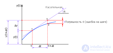
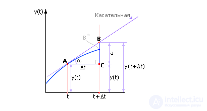
Consider again this important relation, deriving it from geometrical considerations (Fig. 10.3).
|
|
| Fig. 10.3. Geometric illustration of the Euler method |
Let A be the point at which the state of the system is known. This is the “real” state of the system.
At point A to the trajectory of the system, draw a tangent. The tangent is the derivative of the function f ( x ( t ), y ( t ), t ) with respect to the variable t . It is always easy to calculate the derivative at a point; it is enough to substitute the known variables (at the moment “Present” they are known) into the formula y ' = f ( x ( t ), y ( t ), t ).
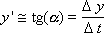
Note that, by definition, the derivative is related to the angle of inclination of the tangent: y ' = tg ( α ), which means that the angle α is easy to calculate ( α = arctan ( y ' )) and draw a tangent.
Draw a tangent to the intersection with the line t + Δ t . The moment t + Δ t corresponds to the “future” state of the system. Draw a line parallel to the t axis from point A to the intersection with the line t + Δ t . The lines form a right triangle ABC, one leg of which is Δ t (known). The angle α is also known. Then the second leg in the right triangle ABC is: a = Δ t · tg ( α ). Now it is easy to calculate the ordinate of point B. It consists of two segments - y ( t ) and a . The ordinate symbolizes the position of the system at the point y ( t + Δ t ). That is, y ( t + Δ t ) = y ( t ) + a or further y ( t + Δ t ) = y ( t ) + Δ t · tg ( α ) or, substituting further, we have: y ( t + Δ t ) = y ( t ) + Δ t · y ' and, finally, y ( t + Δ t ) = y ( t ) + Δ t · f ( x ( t ), y ( t ), t ). Again we obtained the Euler formula (from geometrical considerations).
This formula can give accurate results only for very small Δ t (they say when Δ t is> 0). When Δ t ≠ 0, the formula gives a discrepancy between the true value of y and the calculated one, equal to ε , therefore, it should have an approximate equality sign, or it should be written as:
y ( t + Δ t ) = y ( t ) + Δ t · f ( x ( t ), y ( t ), t ) + ε .
And in fact. Take another look at pic. 10.3. We will mentally move the line t + Δ t to the left (in fact, we will bring the value of Δ t to zero). It is easy to see that the distance BB * = ε , - that is, an error! - will shrink. In the limit (at Δ t -> 0) the value of the error ε will be zero.
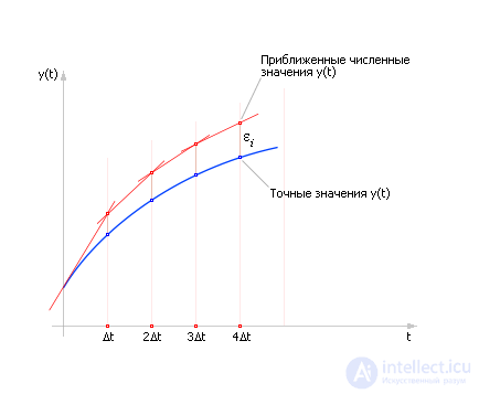
So, replacing the real curve of a straight line (tangent) on the segment Δ t , we introduce an error into the solution, as a result not getting to the point “2” (see. Fig. 10.2), but to the point, to the point “3”. Obviously, this numerical method at each step has an error in calculating ε .
It can be seen from the figure that the smaller the value of Δ t is taken, the smaller the error in calculating ε will be. That is, to calculate the behavior of the system for any lengthy period of time (for example, from t 0 to t k ), in order to reduce the error at each step, the steps Δ t are made as small as possible. To reach the point t k, the segment ( t k - t 0 ) is divided into segments of length Δ t ; thus, the total will be N = ( t k - t 0 ) / Δ t steps. As a result, the calculation will have to apply the Euler formula for each step, that is, N times. But it should be borne in mind that the errors ε i at each i- th step (in the simplest case) are added up, and the total error accumulates quickly (see Fig. 10.4). And this is a significant drawback of this method. Although using this method you can get (in numerical form) the solution of any differential equation (including analytically unsolvable). By reducing the step, we get more accurate solutions, but we should not forget that an increase in the number of steps leads to computational costs and a decrease in speed. In addition, with a large number of iterations, another significant error is introduced into the calculation due to the limited accuracy of the computers and rounding errors.
|
|
| Fig. 10.4. Increasing the total error in the Euler method on a number of steps |
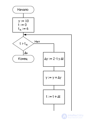
Task 1. Given the differential equation y ' = 2 t y . The initial position of the system is given: y (0) = 1. It is required to find y ( t ), that is, the behavior of the system on the time interval t from 0 to 1.
y ' = 2 t y .
By the method of separation of variables we find:
y ' / y = 2 t
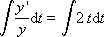
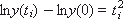
We will integrate from 0 to t i , then according to the rules of integration we have:

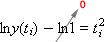

The resulting analytical solution is characterized by the fact that it is absolutely accurate, but if the equation turns out to be somewhat complicated, then the solution will not be found at all. The analytical solution is not universal.
The numerical method of solution assumes that the calculation will be carried out according to the Euler formula in a series of successive steps. At each step, the solution has its own error (see Fig. 10.2), since at each step the curve is replaced by a straight line segment.
In an algorithmic implementation, the calculation is implemented by a cycle in which t (counter t ) and y changes:
|
The block diagram for the implementation of the method on a computer is shown in Fig. 10.5.
|
|
| Fig. 10.5. Block diagram of the implementation of the Euler method |
In the implementation of the Stratum record will look like this (the presence of the symbol "~" at t ):
|
We will look for the value of y of the example considered earlier in numerical form on the interval from T = 0 to T = 1. Take the number of steps n = 10, then the increment step Δ t will be: Δ t = (1 - 0) / n = (1 - 0 ) / 10 = 0.1.
| Table 10.1. Numerical calculation of the equation by the Euler method and comparing the result with the exact solution at each step |
||||||||||||||||||||||||||||||||||||||||||||||||||||||||||||||||||||||||||||||||||||
|
Note that the calculated numerical value ( y i + 1 ) is different from the exact one ( y is exact . ), And the error (the difference between the columns y i + 1 and y is exact. ) Increases in the calculation process just as shown in Figure . 10.4.
Now we calculate the relative error σ for the calculated value of y (1), obtained numerically, in comparison with the theoretical exact y theory. according to the following formula:
σ = (1 - y calc. / y theory. ) · 100%
and compare σ for different values of Δ t .
If we change the value of the step Δ t , for example, decrease the step, then the relative error of the calculation will also decrease. This is what happens when calculating the y (1) value with different step values (see Table 10.2).
| Table 10.2. Dependence of error calculation of step size Δ t |
||||||||||||||||
|
As you can see, with a decrease in the increment step Δt , the value of the relative error decreases, which means that the accuracy of the calculation increases.
Please note that a step change of 10 times (from 1/10 to 1/100) leads to a change in the magnitude of the error about 10 times as well (from 14% to 2%). If you change the pitch 100 times, the error will also decrease by about 100 times. In other words, the step size and error for the Euler method are linearly related. If you want to reduce the error by 10 times - reduce the step by 10 times and increase the number of calculations accordingly by 10 times. In mathematics, this fact is usually denoted by the symbol ε = O (Δ t ), and the Euler method is called the first-order method of accuracy.
Since in the Euler method the error is sufficiently large and accumulates from step to step, and the accuracy is proportional to the number of calculations, the Euler method is usually used for rough calculations, for evaluating the behavior of the system in principle. For accurate quantitative calculations apply more accurate methods.
Notes
Set out in paragraphs. 1-4 we will explain on an example.
Example. Let be
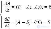
Qualitatively, these equations describe the process of heat exchange between two bodies, the temperatures of which at some time point are denoted as A and B. In general, A and B are variables that vary in time t . Finding the behavior of the system means that you need to find out how the temperatures A ( t ) and B ( t ) will change.
It is intuitively clear that with the initial temperature difference A = 8 and B = 5, the temperatures of the bodies should gradually equalize over time, since the hotter body will give off energy to the colder one, and its temperature will decrease, and the colder body will receive the energy from the hotter and its temperature will increase. The heat exchange process will end (that is, the changes will stop) when the temperatures of the two bodies become the same.
We will carry out several calculations of the behavior of A ( t ) and B ( t ) with different step sizes Δ t .
We will take a different step size Δ t and find the corresponding values of A and B in time using the following Euler formulas:
A new. = A prev. + ( B prev. - A prev. ) · Δ t ,
B new = B prev. + ( A prev. - B prev. ) · Δ t .
Calculation at Δ t = 2 (tab. 10.3).
| Table 10.3. Temperature change bodies in numerical calculation with step 2 |
||||||||||||||||
|
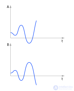
There is a phenomenon of “razboltki” (see. Fig. 10.6). An unsustainable solution. From physical considerations it is obvious that two bodies cannot behave this way during heat exchange.
|
|
| Fig. 10.6. The system behaves well wrong. The solution is unstable |
Calculation at Δ t = 1 (tab. 10.4).
| Table 10.4. Temperature change bodies in numerical calculation with step 1 |
||||||||||||||||
|
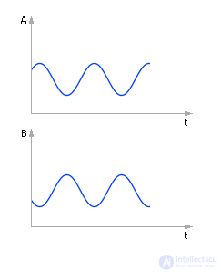
The behavior of the solution of the system at the stability boundary is observed (see Fig. 10.7).
|
|
| Fig. 10.7. The system behaves well wrong. The solution is on the verge of sustainability. |
Calculation at Δ t = 0.5 (tab. 10.5).
| Table 10.5. Temperature change bodies in numerical calculation in 0.5 steps |
||||||||||||||||
|
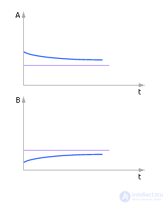
The solution is stable, corresponds to the correct qualitative picture (see fig. 10.8). The temperature of the bodies gradually converge, becoming the same over time. But the solution so far has a large error.
|
|
| Fig. 10.8. The system behaves qualitatively correctly. The solution (system behavior) has a large error. |
Calculation at Δ t = 0.1 (tab. 10.6).
| Table 10.6. Temperature change bodies in numerical calculation in 0.1 steps |
||||||||||||||||||||||||||||
|
The solution is stable. The solution is more accurate (see fig. 10.9).
|
|
| Fig. 10.9. The system behaves qualitatively correctly. Quantify the solution more accurately |
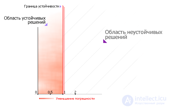
The role of changing the step size is illustrated in Fig. 10.10.
|
|
| Fig. 10.10. The relationship of the magnitude of the calculation step with the stability of the method and its accuracy (for example) |


Comments
To leave a comment
System modeling
Terms: System modeling